Introduction to Flat-Top Pulse-Amplitude Modulation

Pulse amplitude modulation (PAM) may be implemented either through natural sampling or with flat‑top pulses. Last time, we explored the key properties of natural sampling PAM, including its spectrum and the recovery of the message signal. Now, we turn to flat-top PAM. After introducing the flat-top PAM waveform and its generation using a sample-and-hold circuit, we’ll provide a detailed derivation of its frequency spectrum. This mathematical derivation lays the foundation for understanding the aperture effect distortion and message recovery, topics that will be discussed in great detail in the next article.

 

Natural Sampling vs. Flat-Top PAM

As shown in Figure 1, natural‑sampling PAM preserves the shape of the message signal during each pulse.

 

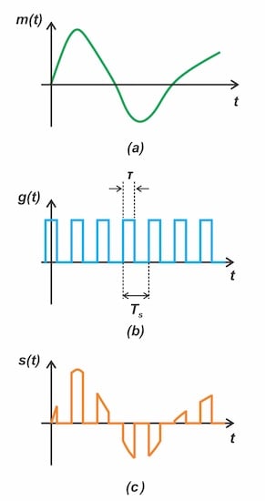
Figure 1. (a) Message signal; (b) rectangular switching waveform; (c) naturally‑sampled PAM waveform.

 

This modulation scheme transmits equally spaced time slices of the message signal. Put differently, the message signal is multiplied by a carrier g(t) that takes the form of a pulse train, rather than the continuous sinusoidal wave used in amplitude modulation (AM).

According to the sampling theorem, recovery of the message signal m(t) from its samples depends not on the slice duration τ, but on the sampling frequency 2π / T_s, which must be greater than twice the highest frequency present in m(t). This implies that the exact shape of the sampling pulse is not fundamental to the scheme’s operation; what matters most is transmitting the discrete samples of the message.

Although PAM may be realized with various pulse forms, flat‑top PAM is a commonly used practical choice: it maintains the sampled amplitude throughout the pulse duration τ, which makes certain aspects of the circuit implementation more straightforward. Figure 2 illustrates the message signal alongside its corresponding flat‑top PAM waveform.

 

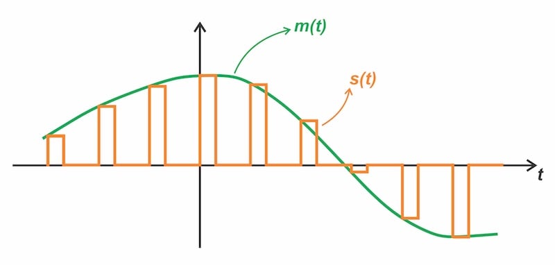
Figure 2. Message signal (green) and the corresponding PAM waveform (orange).

 

In the sections that follow, our discussion centers on flat‑top PAM. For brevity, PAM without a qualifier will denote flat‑top PAM rather than natural‑sampling PAM unless otherwise stated.

 

Generation of Flat-Top PAM

The generation of a PAM signal can be conceptually understood as a two‑step process. First, the message signal m(t) is instantaneously sampled every T_s seconds, with the sampling rate f_s = 1 / T_s chosen according to the sampling theorem. Second, each discrete sample is extended in time to a fixed duration τ, producing a sequence of pulses whose amplitudes match the sampled values of the original signal.

Although this is described as a two‑step process, in practice both operations are carried out simultaneously by a single circuit known as the sample‑and‑hold. A basic sample‑and‑hold circuit for generating a flat‑top PAM waveform is implemented using two FET switches and a capacitor, as shown in Figure 3.

 

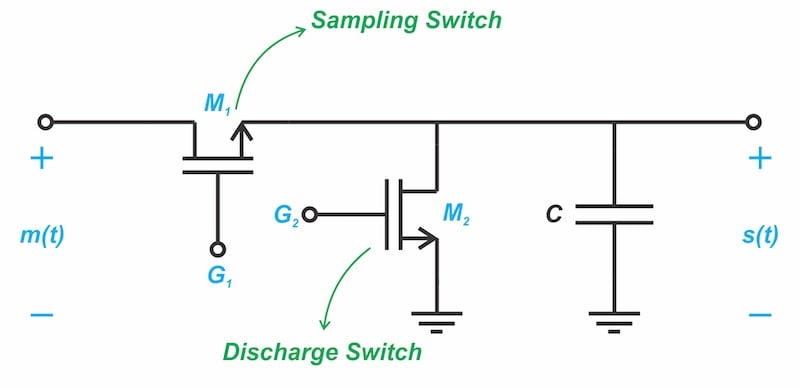
Figure 3. Sample‑and‑hold circuit for generating flat‑top PAM.

 

The operation of the circuit can be described as follows: A short pulse applied to the sampling switch M₁ charges the capacitor to the instantaneous input voltage. When M₁ opens, the capacitor holds this value for τ seconds. A subsequent pulse then activates the discharge switch M₂, allowing the capacitor to return to zero volts.

In the rest of the article, we’ll work out the spectrum of flat‑top PAM, which will help us understand its properties and how the message can be recovered. But first, we’ll revisit a few essential signals and systems concepts.

 

Relevant Fourier Tools for PAM Analysis

Because Fourier properties and identities can be easy to forget or mix up, this section provides a concise review of the concepts most relevant to PAM, giving readers a solid reference point to follow the discussion. The first concept to establish is the impulse train with period T_s, where impulses appear once every T_s seconds, as illustrated in Figure 4.

 

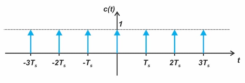
Figure 4. Impulse train with period T_s.

 

An operation fundamental to the PAM scheme is instantaneous sampling, which is achieved by multiplying the input signal with an impulse train. Hence, understanding the Fourier transform of the impulse train is essential. In the time domain, the impulse train may be expressed by an infinite summation:

$$c(t) = \sum_{n=- \infty}^{+ \infty} \delta(t-nT_s)$$

Equation 1.

 

How do we find the Fourier transform of this signal? Since the impulse train is a periodic signal with period T_s, we first compute its Fourier series coefficients, which all equal 1 / T_s. Recall that the Fourier transform of a periodic signal is given by its Fourier series coefficients multiplied by impulses at integer multiples of the fundamental frequency f_s = 1 / T_s. Thus, the transform of the impulse train becomes:

$$C(f) = \frac{1}{T_s} \sum_{k=- \infty}^{+ \infty} \delta(f- \frac{k}{T_s})$$

Equation 2.

 

This means the spectrum consists of impulses spaced at multiples of the sampling frequency f_s = 1 / T_s, each scaled by 1 / T_s, as shown in Figure 5(a).

 

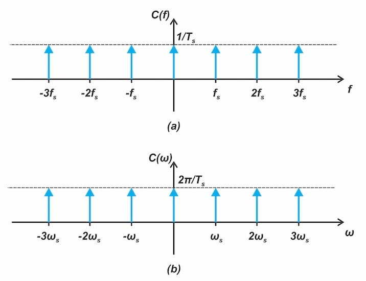
Figure 5. Fourier transform of the impulse train shown versus frequency in hertz (a) and angular frequency (b).

 

Note that when expressed in terms of angular frequency ω rather than f measured in hertz, the Fourier transform of the impulse train becomes another impulse train with impulses spaced at multiples of ω_s = 2π / T_s and scaled by 2π / T_s, instead of being scaled by 1 / T_s. Figure 5(b) shows the transform against ω. Throughout the rest of the article, we’ll represent Fourier transforms using frequency f measured in hertz.

Another important Fourier transform property for PAM analysis is that convolving two time-domain functions x(t) and y(t) corresponds to multiplying their frequency-domain transforms X(f) and Y(f). Mathematically, we have:

$$z(t) = x(t) * y(t) \overset{\mathcal{F}}{\longleftrightarrow} Z(f) = X(f) Y(f)$$

Equation 3.

 

On the other hand, when two signals x(t) and y(t) are multiplied in the time domain, their spectra are convolved in the frequency domain. Formally:

$$z(t) = x(t) \, y(t) \overset{\mathcal{F}}{\longleftrightarrow} Z(f) = X(f) * Y(f)$$

Equation 4.

 

Alright, with the Fourier overview out of the way, let’s dive into PAM.

 

Deriving the Time‑Domain Expression for PAM

We first develop the time‑domain representation of the PAM waveform. In the time domain, a PAM signal can be viewed as a train of pulses, each scaled by the amplitude of the corresponding signal sample. Let p(t) denote the unit-amplitude pulse centered at the origin, as shown in Figure 6.

 

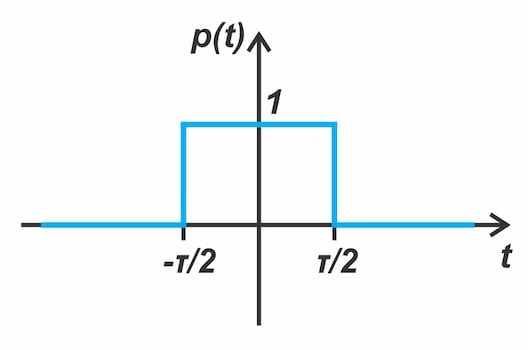
Figure 6. Unit‑amplitude pulse p(t) centered at the origin.

 

The pulse occurring at nT_s is then p(t − nT_s). The complete pulse train is therefore a sum of these shifted replicas and can be written as:

$$g(t) = \sum_{n=-\infty}^{\infty} p\! \left(t - nT_s\right)$$

Equation 5.

 

Because the pulse at nT_s is weighted by the corresponding message sample m(nT_s), the resulting flat-top PAM signal may be expressed as:

$$s(t) = \sum_{n=-\infty}^{\infty} m\! \left(nT_s \right) \, p\! \left(t - nT_s\right)$$

Equation 6.

 

To facilitate the derivation of the modulated signal’s spectrum, we rewrite s(t) in a more tractable form. The essential property that we’ll use is that convolution with a delayed delta function results in a corresponding delay of the signal. For example, convolving x(t) with δ(t − t₀) yields the time‑shifted signal x(t − t₀). By invoking this property, the pulse located at nT_s may be expressed as:

$$p(t - nT_s) = p(t) * \delta(t - nT_s)$$

Equation 7.

 

Therefore, the modulated signal (Equation 6) becomes:

$$s(t) = \sum_{n=-\infty}^{\infty} m\! \left(nT_s \right) \, \bigg ( p(t) * \delta(t - nT_s) \bigg)$$

Equation 8.

 

Finally, extracting p(t) from the summation yields:

$$s(t) = p(t) * \sum_{n=-\infty}^{\infty} m\! \left(nT_s \right) \, \delta(t - nT_s)$$

Equation 9.

 

This form is particularly convenient for spectral analysis, as convolution in the time domain corresponds to multiplication in the frequency domain (see Equation 3), and the functions involved have well‑known Fourier transforms.

 

Fourier Transforms of the PAM Constituent Functions

With Equation 9 in hand, we now derive the Fourier transform of the modulated signal, which is given by:

$$S(f) = P(f) \times \mathcal{F} \bigg ( \sum_{n=-\infty}^{\infty} m\! \left(nT_s \right) \, \delta(t - nT_s) \bigg )$$

Equation 10.

 

Here, P(f) denotes the Fourier transform of p(t), while the second term on the right‑hand side corresponds to the transform of the summation component. The transform of p(t) is achieved by directly applying the Fourier transform definition. As shown in Figure 6, p(t) is a rectangular pulse whose high portion occupies the interval −τ / 2 ≤ t ≤ τ / 2 and is zero elsewhere. Therefore, we have:

$$P(f) = \int_{-\tau/2}^{\tau/2} e^{-j2\pi f t}\, dt = \frac{\sin(\pi f \tau)}{\pi f} = \tau\,\mathrm{sinc}(\pi f \tau)$$

Equation 11.

 

where sinc(x) = sin x / x.

The next step is to determine the Fourier transform of the summation term appearing in Equation 10. This term, denoted by m_s(t) in the rest of the article, is simply an impulse train weighted by the sample values. To aid intuition, Figure 7 depicts a representative time‑domain signal m(t) together with the corresponding weighted impulse train m_s(t).

 

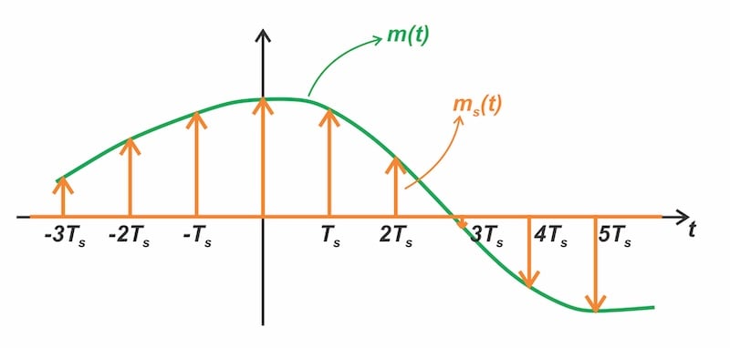
Figure 7. The message signal m(t) and its instantaneously sampled version m_s(t).

 

The instantaneously sampled version m_s(t) is obtained by multiplying m(t) by a unit‑amplitude impulse train of period T_s. What spectrum results from this operation? The plots in Figure 8 help clarify the effect.

 

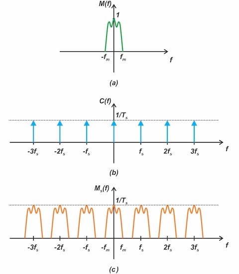
Figure 8. Multiplying a signal by an impulse train leads to replicas of the input spectrum at multiples of the sampling frequency.

 

Figure 8(a) shows the representative message spectrum, whose highest frequency component is f_m. Figure 8(b) illustrates the spectrum corresponding to a unit‑amplitude impulse train of period T_s. As discussed earlier, a periodic impulse train in time becomes a periodic impulse train in frequency where the spacing in frequency is the fundamental frequency f_s = 1 / T_s and the amplitude of each spectral impulse is 1 / T_s.

When m(t) is multiplied by the impulse train in the time domain to produce m_s(t), their spectra shown in Figures 8(a) and 8(b) are convolved in the frequency domain (See Equation 4). Furthermore, we know that convolving a spectral component with a shifted delta function moves the spectral component to the delta function’s location. Therefore, the spectrum of m_s(t) consists of replicas of the message spectrum at integer multiples of the sampling frequency, as illustrated in Figure 8(c).

 

Putting It Together: Spectrum of Flat-Top PAM

Figure 9 illustrates the spectrum of the instantaneously sampled signal M_s(f) and the magnitude of P(f) for τ = T_s.

 

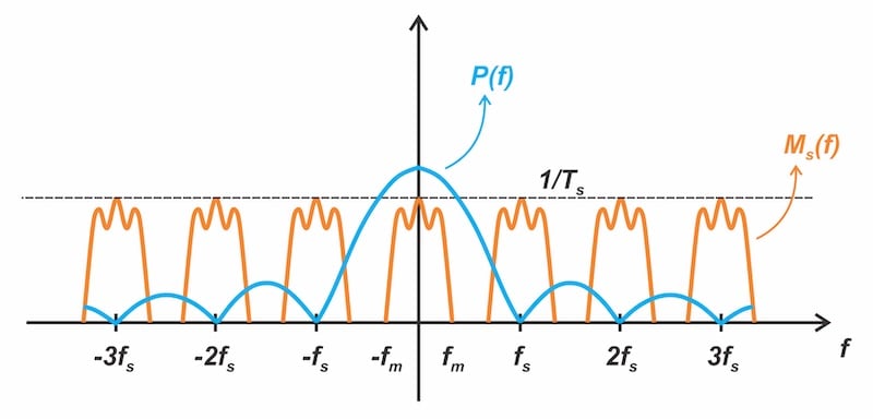
Figure 9. Magnitudes of the Fourier transforms of the PAM constituent functions.

 

Now that we have P(f) and M_s(f), multiplying them gives the spectrum of the modulated signal. Figure 10 shows how this spectrum appears at frequencies below f_s / 2.

 

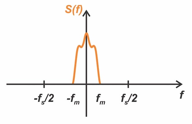
Figure 10. Illustrative spectrum of s(t) at frequencies below f_s/2, derived from the assumed message spectrum.

 

The key observation is that the sinc function does not exhibit a flat spectrum across the message bandwidth. As a result, higher‑frequency components of the message spectrum are attenuated relative to those near DC. Figure 10 illustrates this effect, showing reduced peaking in the higher‑frequency region of the assumed message spectrum. This non‑uniform response highlights the potential for distortion in the flat-top PAM method.

Put differently, flat‑top sampling can be viewed as passing the sampled signal m_s(t) through a system with transfer function P(f). Since P(f) rolls off at high frequencies, it acts as a low‑pass filter that suppresses the upper portion of the message spectrum. This distortion, known as the aperture effect, introduces a known, predictable weighting to the signal’s spectrum. Consequently, the distortion can be compensated by an equalization filter that amplifies the high-frequency portion of the spectrum in a way that counteracts the loss from the aperture effect. In the next article, we’ll explore distortion in PAM signals in greater detail and further elaborate on the equalization technique.

 

Wrapping Up

In this article, we derived the spectrum of flat-top PAM. Flat-top PAM maintains the sampled amplitude throughout the pulse duration τ. In the time domain, a PAM signal can be viewed as a train of pulses, each scaled by the amplitude of the corresponding signal sample. A key limitation of flat-top PAM is the aperture effect distortion, which can be mitigated by an equalization filter. While this article focused on deriving the spectrum, the next article will examine the aperture effect and its equalization in greater detail.