Learn How Integrated Solutions Can Increase the Accuracy of Resistive Current Sensing

A discrete amplifier along with some external gain-setting resistors can be used to gain up the voltage across a current sense resistor. Although such discrete solutions can be cost-effective, they cannot offer a high accuracy because of the limited matching of the external components. The attempt to use a high-accuracy resistor network can offset the cost savings one might expect from using a simple discrete solution.

Discrete Implementations for Resistive Current Sensing

In a previous article, we discussed that the op-amp-based non-inverting configuration can be used to sense and gain up the voltage across a low-side current sense resistor. The non-inverting configuration has a single-ended input and senses its input voltage with respect to ground. That’s why we cannot use this amplifier in a high-side sensing configuration.

On the other hand, the classical difference amplifier has a differential input. Since it senses the voltage drop across the shunt resistor rather than the voltage of a node with respect to ground, it can be used for both low-side and high-side current sensing applications as shown in Figure 1.

In this article, we’ll discuss two of the important error sources that can affect the accuracy when using a difference amplifier.

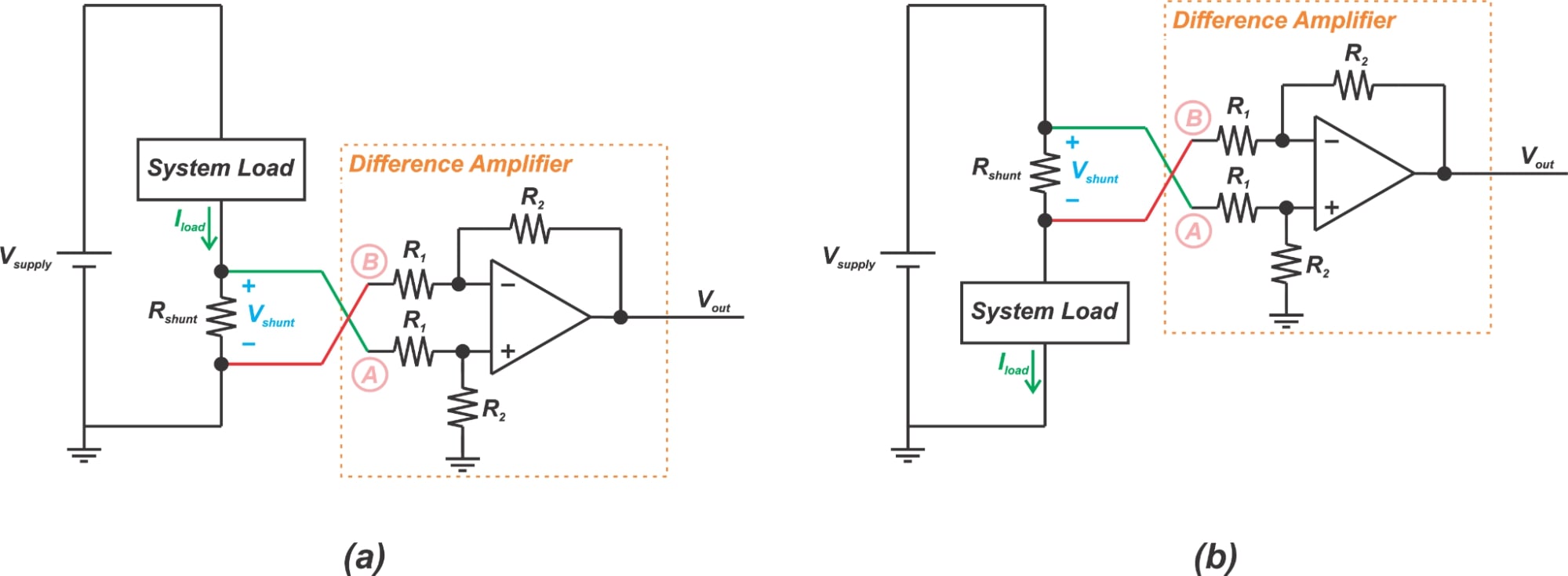
Figure 1. Using a difference amplifier in (a) low-side and (b) high-side current sensing.

Common-Mode Rejection Ratio: A Key Feature

Common-mode rejection ratio is the ability of a differential input amplifier to reject signals that are common to both inputs. The transfer function of an amplifier can be expressed as:

\[v_{out}=A_{dm}v_{d}+A_{cm}v_{c}\]

Equation 1.

where \(A_{dm}\) and \(v_{d}\) are respectively the differential-mode gain of the amplifier and the differential signal at the amplifier input. Similarly, \(A_{cm}\) and \(v_{c}\) are the common-mode gain and the common-mode signal applied to the amplifier. According to Equation 1, the voltage that appears at the amplifier output is a function of the common-mode value of the input. In Figure 1(b), we ideally expect the output to be a function of the differential signal V_shunt. However, in reality, the output is also a function of the supply voltage V_supply.

As we change V_supply, the common-mode signal at the amplifier input and consequently, the output voltage of the amplifier changes. This happens even if we keep V_shunt constant. To reduce this non-ideal effect, we need to make the common-mode gain A_cm much smaller than the differential-mode gain A_dm. The common-mode rejection ratio (CMRR), defined as the differential gain divided by the common-mode gain, specifies the ability of an amplifier to reject common-mode signals while amplifying differential signals.

Discrete Implementations Have a Low CMRR

Consider the difference amplifier shown in Figure 2.

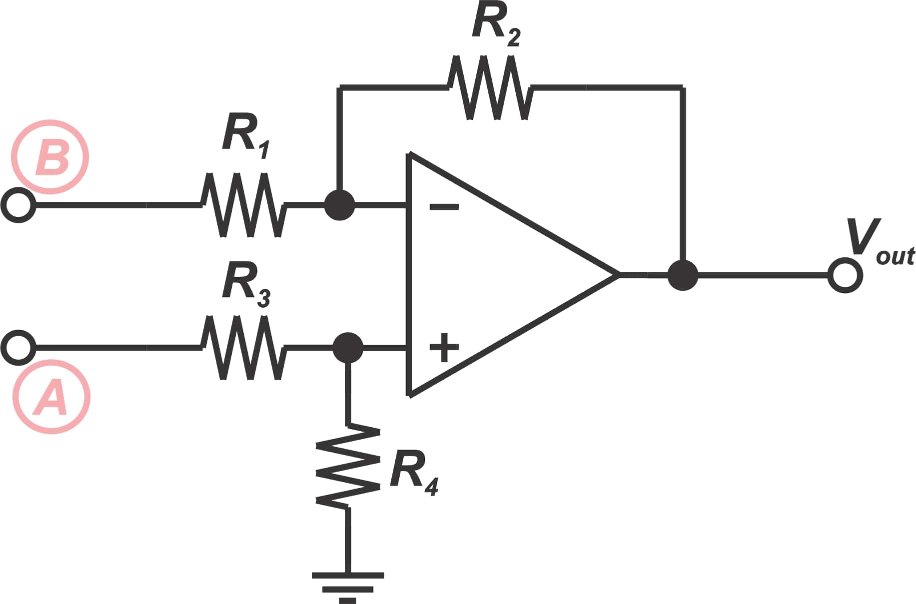
Figure 2.

With an ideal op-amp, the transfer function of the difference amplifier is given by:

\[v_{out}=\frac{R_{4}}{R_{1}}\times\frac{R_{1}+R_{2}}{R_{3}+R_{4}}\times v_{A}-\frac{R_{2}}{R_{1}}\times v_{B}\]

For \(\frac{R_{2}}{R_{1}}=\frac{R_{4}}{R_{3}}\), we have:

\[v_{out}=\frac{R_{2}}{R_{1}}\left(v_{A}-v_{B}\right)\]

Equation 2.

This equation shows that any common-mode voltage will be completely suppressed by the amplifier, i.e. with \(v_{A}=v_{B}\), we have \(v_{out}=0\). However, in practice, common-mode rejection of a difference amplifier will be limited because the ratio \(\frac{R_{2}}{R_{1}}\) won’t be exactly equal to \(\frac{R_{4}}{R_{3}}\). It can be shown that the CMRR of a difference amplifier is given by:

\[CMRR\simeq \frac{A_{d}+1}{4_{t}}\]

Equation 3.

where \(A_{d}\) is the differential gain of the difference amplifier which is equal to \(\frac{R_{2}}{R_{1}}\); and t is the resistor tolerance. For example, with a differential gain of 1 and 0.1% resistors, we have:

\[CMRR\simeq\frac{A_{d}+1}{4_{t}}=\frac{1+1}{4\times0.001}=500\]

Expressing this value in dB, we get a CMRR of about 54 dB. Note that Equation 3 is derived based on the assumption that the op-amp is ideal and has a very high CMRR. If the CMRR of the op-amp is not much larger than the value obtained from Equation 3, we’ll need to use a more complicated equation.

Integrated Solutions Can Lead to a High CMRR

Hence, even with an ideal op-amp, the CMRR of a difference amplifier is relatively low and limited by the matching of the gain-setting resistors. To combat this problem, we can use an array of matched resistor networks such as the LT5400. The LT5400 is a  quad resistor network with an excellent matching of 0.005% and can be used to create difference amplifiers with a high CMRR, as shown in Figure 3. Using matched resistor networks, a CMRR of about 80 dB should be achievable.

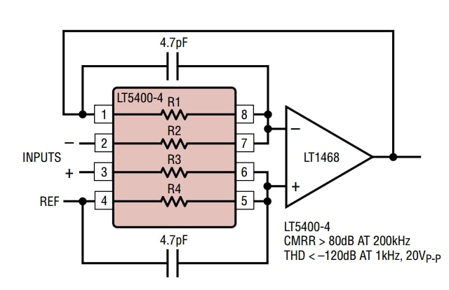
Figure 3. Resistor arrays can be used to create difference amplifiers with very high CMRR. Image used courtesy of Linear Technology

A discrete amplifier along with some external gain-setting resistors might be considered as a low-cost current measurement solution. However, as you can see, the matching of the gain-setting resistors determines the CMRR of the amplifier. The attempt to use a separate high-accuracy resistor network can offset the cost savings one might expect from using a simple difference amplifier.

Rather than using a precision op-amp along with a separate resistor network, we can use a completely monolithic solution such as the AMP03 from Analog Devices that integrates laser-trimmed resistors into the precision op-amp package to achieve a high matching between the resistors. Such integrated solutions can obtain a CMRR greater than 100 dB.

Another Error Source: the Temperature Drift of the Gain-Setting Resistors 

The temperature drift of the gain-setting resistors is another factor that can affect measurement accuracy. As discussed above, the tolerances of the gain-setting resistors determine the initial accuracy of the amplifier at room temperature. However, for the resistor ratios to be constant, the resistors should exhibit similar behavior over the operating temperature range.

To better understand how temperature drift can produce a gain error, let’s consider an example. Assume that the resistor values in Equation 2 are R1=5 kΩ and R2=100 kΩ. Also, suppose that the temperature coefficient of the resistors is ±50 ppm/°C and the ambient temperature can go 100 °C above the reference temperature (the room temperature).

What is the maximum and minimum value of the differential gain \(\frac{R_{2}}{R_{1}}\)?

A 100 °C temperature rise above the reference temperature can change the value of a ±50 ppm/°C resistor by ±0.5 %. Hence, the maximum differential gain is given by:

\[A_{dm, max}=\frac{R_{2,max}}{R_{1,min}}=\frac{100\times(1+0.005)}{5\times(1-0.005)}=20.20\]

The minimum gain is obtained by:

\[A_{dm, max}=\frac{R_{2,min}}{R_{1,max}}=\frac{100\times(1-0.005)}{5\times(1+0.005)}=19.80\]

Note that the resistors can drift in opposite directions. In this example, 1% of gain error is caused only by the drift effect as we assume that the resistors have their nominal value at room temperature.

Interestingly, with a matched resistor network such as the LT5400 or a completely monolithic current sense solution, the integrated resistors can exhibit near-perfect matching of both the initial error as well as the temperature drift. This is illustrated in Figure 5.

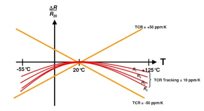
Figure 5. Image used courtesy of Vishay

In this figure, the orange lines specify the limits for the change in the value of a single ±50 ppm/°C resistor as temperature changes in either direction from the reference temperature (20°C). The red curves specify the temperature behavior of four integrated resistors of a matched resistor array.

While a single resistor from the matched resistor network can exhibit a temperature coefficient of ±50 ppm/°C, the temperature behavior of the four integrated resistors is very well-matched. The resistor values track each other as the temperature changes. These matched resistors allow us to keep the amplifier gain relatively constant over the operating temperature range.

Conclusion

A discrete amplifier along with some external gain-setting resistors can be used to gain up the voltage across a current sense resistor. Although such discrete solutions can be cost-effective, they cannot offer a high accuracy because of the limited matching of the external components.

The matching of the gain-setting resistors determines the CMRR of the amplifier. Near-perfect matching of both the initial error as well as the temperature drift of the resistors is required to achieve a high CMRR. That’s why integrated solutions can easily defeat discrete implementations in terms of CMRR. Note that the attempt to use a separate high-accuracy resistor network can offset the cost savings one might expect from using a simple discrete solution.

To see a complete list of my articles, please visit this page.