Non-Uniform Quantization in PCM: Comparing μ-Law and A-Law Compression

Analog voice signals exhibit a non-uniform amplitude distribution, characterized by frequent low-amplitude segments interspersed with occasional large excursions. Because of this non-uniform distribution, the use of uniform quantization generates significant quantization noise in voice applications. To address this limitation, non-uniform quantization uses tapered quantizing levels, where smaller steps are used for low amplitudes and progressively larger steps for higher amplitudes.

As discussed in the previous article, non-uniform quantization improves SNR during soft utterances. In this article, we’ll compare uniform and non-uniform quantization through numerical examples to further clarify the operation of the non-uniform method. We’ll then examine two commonly used compression characteristics, namely the μ-Law and A-Law methods. Finally, we’ll briefly discuss implementation methods for the compression function.

 

Further Insight into Non-Uniform Quantization

In the previous article, we used the representative speech signal in Figure 1 to demonstrate how non-uniform quantization can reduce quantization noise for signals with non-uniform amplitude distribution.

 

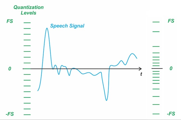
Figure 1. Using uniform and non-uniform quantization for a representative speech signal.

 

Because smaller amplitudes dominate statistically, non-uniform quantization allocates more finely spaced levels in this region to better match the signal’s behavior. In contrast, a uniform quantizer wastes many levels on rare peaks and provides too few where the signal spends most of its time. This leads to poor resolution and higher distortion in soft speech segments. By allocating smaller steps for low amplitudes and larger steps for high amplitudes, non-uniform quantization aligns the quantizer’s resolution with the actual amplitude distribution of speech, improving the overall SNR performance.

Comparing numerical examples of uniform and non-uniform quantization further clarifies the operation of the non-uniform method. To illustrate the concept, we compare two quantizers. The uniform quantizer has all integer levels from 0 to 8. The non-uniform quantizer has progressively expanding steps, with quantization levels of 0, 1, 2, 4, and 8, as shown in Figure 2.

 

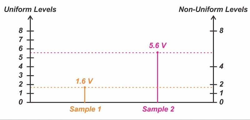
Figure 2. Comparison of uniform and non-uniform quantization.

 

Consider the quantization of Sample 1 with a value of 1.6 V. Since the nearest quantization level for both uniform and non-uniform methods is 2 V, both systems introduce a quantization error of 2 - 1.6 = 0.4 V. Relative to the actual sample value, this corresponds to an error of (0.4 / 1.6) × 100% = 25%.

For Sample 2 with a value of 5.6 V, the nearest quantization level in the uniform system is 6 V. This yields an absolute error value of 0.4 V, or a relative error of (0.4 / 5.6) × 100% = 7.1%. In the non-uniform system, however, the nearest level is 4 V, resulting in an absolute error of 1.6 V and a relative error of (1.6 / 5.6) × 100% = 28.6%. Table 1 summarizes the results of these calculations.

 

Table 1. Summary of relative error calculations for uniform and non-uniform quantizers.

	Uniform Quantization	Non-Uniform Quantization
Sample 1 (1.6 V)	25%	25%
Sample 2 (5.6 V)	7.1%	28.6%

 

For these example values, the relative error of the uniform method falls from 25% at low amplitudes to 7.1% at high amplitudes. Since the step size remains constant, the relative error diminishes at higher amplitudes. In contrast, the relative error of the non-uniform method changes from 25% to 28.6%, showing much smaller variation. This stability occurs because the quantizer’s step sizes increase at higher amplitudes, resulting in an almost constant relative error.

In summary, while the non-uniform quantizer exhibits a larger absolute quantization error at high amplitudes, its relative (percentage) error remains nearly constant. A comparison of the two quantizers examined above shows that the non-uniform method requires fewer quantization levels overall, which helps reduce the word length in digital systems.

Most applications involve quantizing signals with a relatively uniform amplitude distribution, where the signal spends most of its time at medium or high amplitudes. In such cases, a uniform quantizer is typically used, as it exhibits relatively small error when the signal amplitude is not low.

In contrast, voice signals spend most of their time at low amplitudes. Therefore, a non-uniform quantizer is used, which allocates more quantization levels to this region to limit the quantization noise. As shown in the numerical example above, the relative error of the non-uniform quantizer remains almost constant at high amplitudes, even though fewer quantization levels are used there. This strategy achieves a given SNR performance with fewer total quantization levels, ultimately reducing the required word length in PCM systems.

 

μ-Law Compression Characteristic

A particular type of compression characteristic that is often used in practice is the so-called μ-law characteristic, defined by:

$$y=sgn(x) \; \frac{ln (1+ \mu |x|)}{ln(1+ \mu)}$$

Equation 1.

where:

ln denotes the natural logarithm

μ is a positive constant that determines the degree of compression.

The variables x and y represent the normalized input and output of the compressor, respectively. The normalized input x is obtained by dividing the message signal m(t) by its peak value m_p. Consequently, the output y also has a peak value of unity. Figure 3 shows the compression characteristic for several values of μ.

 

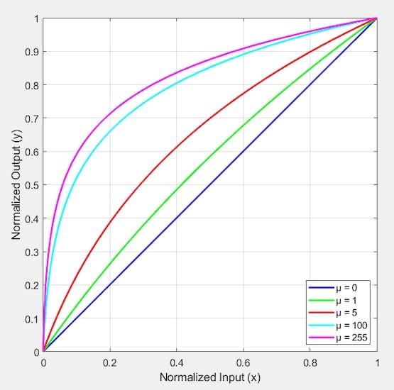
Figure 3. μ-law compression characteristic for several values of μ.

 

The case of μ = 0 corresponds to linear amplification (or uniform quantization). This can be verified by evaluating Equation 1 in the limit as μ approaches zero. To obtain a nearly constant SNR over a dynamic range of 40 dB, μ should be greater than 100. In practice, μ = 255 has been adopted for all North American 8-bit PCM systems.

 

A-Law Compression Characteristic

Another compression characteristic that is used in practice is the so-called A-law characteristic, defined by:

$$y = \begin{cases} sgn(x) \; \frac{A |x| }{1+ln(A)} & 0 \leq |x| \leq \frac{1}{A} \\ sgn(x) \; \frac{1 + ln(A |x| )}{1+ ln(A)} & \frac{1}{A} \leq |x| \leq 1\end{cases}$$

Equation 2.

where:

A is the parameter that determines the level of compression

x and y are the normalized input and output of the compressor.

This equation is plotted in Figure 4 for selected values of A.

 

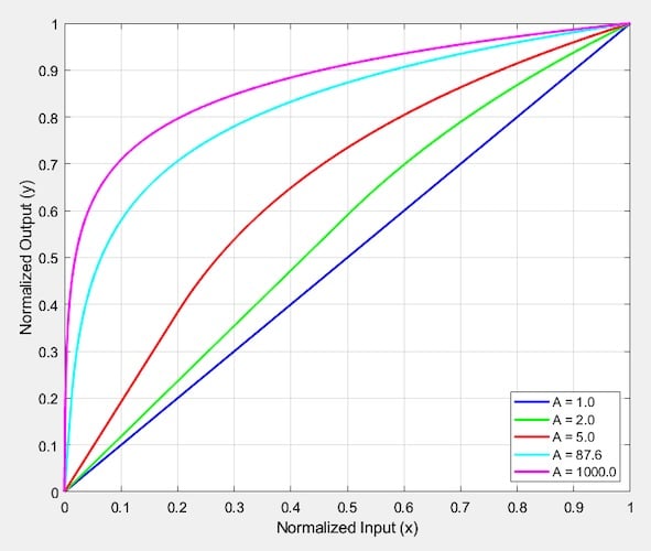
Figure 4. A-law compression characteristic for several values of A.

 

The typical value for A is 87.6, which is standardized and yields results comparable to the μ-law characteristic with μ = 255.

 

Compandor

The compression characteristic applied at the transmitter distorts the signal samples. To restore these samples to their correct relative values, the receiver uses a device with a characteristic complementary to that of the compressor. Figure 5 illustrates representative compression and expansion characteristics. The device with the expansion characteristic is often referred to as an expander.

 

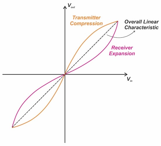
Figure 5. The expander characteristic is the inverse of the compression characteristic.

 

If the compression and expansion laws are exactly the inverse of one another, the expander output will be identical to the compressor input, except for the effects of quantization. The combination of a compressor and an expander is known as a compandor (sometimes spelled compander). Figure 6 illustrates how PCM systems achieve non-uniform quantization by using a compressor followed by a uniform quantizer in the transmitter and an expander in the receiver.

 

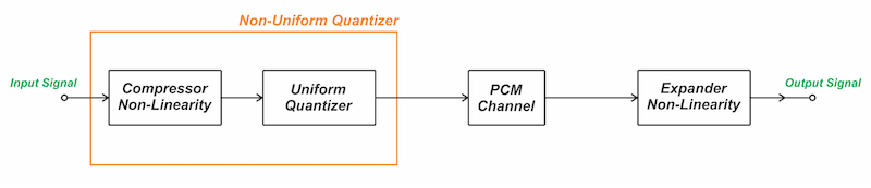
Figure 6. Utilization of compressor and expander for non-uniform quantization.

 

Note that while compressing a signal in the time domain increases its bandwidth, the compression used in PCM doesn’t operate on the timescale. Instead, it compresses only the sample values. Consequently, the issue of increased bandwidth doesn’t arise here.

 

Analog Implementation of Compression Function

Two broad techniques are available for implementing a compressor in PCM applications. One method uses a logarithmic amplifier to realize the compression function, while the second relies on digital circuits. Figure 7 illustrates the analog approach, where a logarithmic amplifier followed by an 8-bit ADC performs non-uniform quantization.

 

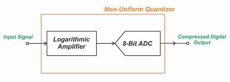
Figure 7. The use of a logarithmic amplifier to implement the compression function.

 

This technique has found use in highly integrated single-chip designs intended for high-volume consumer applications. A logarithmic amplifier may be implemented by means of a semiconductor diode, since the diode’s V-I characteristic exhibits a logarithmic relationship in the first quadrant:

$$V_D= \frac{KT}{q} \; ln \bigg ( 1 + \frac{I_D}{I_s} \bigg )$$

Equation 3.

As illustrated in Figure 8, the logarithmic relationship in the first and third quadrants is obtained by employing two matched diodes in parallel with opposite polarity.

 

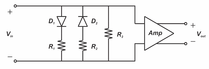
Figure 8. Logarithmic amplifier using biased diodes.

 

The biased-diode configuration represents the simplest type of logarithmic amplifier. While this circuit saw extensive use in the first American PCM telephony system, it presents notable challenges. Specifically, the diodes require careful matching, necessitating trimming after installation. As shown, adjustable resistors are placed in series with each diode and a third variable resistor is added in parallel. By adjusting these resistors, the resulting characteristic is fitted to a finite number of points, usually seven, on the ideal curve. Figure 9 shows the corresponding expansion circuit used in the receiver.

 

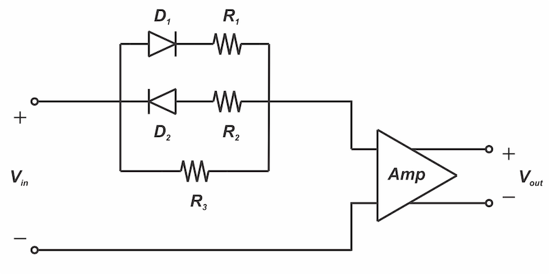
Figure 9. Expansion circuit using biased diodes.

 

Due to the matching difficulties associated with analog implementations, modern systems predominantly employ digital solutions to implement a piecewise linear approximation of the compression curve. The basic concept of this method is shown in Figure 10.

 

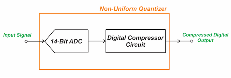
Figure 10. Digital implementation of the non-uniform quantization.

 

In this approach, linear quantization is first carried out by a high-resolution ADC (e.g., 14 bits). The resulting output is subsequently fed to a digital circuit, typically a look-up table, that produces the compressed 8-bit PCM words.

 

Wrapping Up

In this article, we compared uniform and non-uniform quantization through numerical examples and examined the μ-Law and A-Law compression characteristics. Non-uniform quantization can be achieved by passing the input signal through a compressor and then feeding the compressor’s output into a uniform quantizer. This approach effectively compresses the input signal, thereby reducing its dynamic range.

The distortion introduced by this process at the transmitter must be corrected by a complementary expansion operation at the receiver. The combined process of signal compression and expansion is referred to as companding.