Phase Margin Estimation Using the Rate-of-Closure

How can an engineer gauge stability in an analog negative-feedback circuit? For minimum-phase circuits, you can consider using the rate-of-closure.

In everyday analog design, engineers often need to quickly estimate the degree of stability (or lack thereof) of a negative-feedback circuit. A convenient tool that is applicable to minimum-phase circuits (so-called because all their poles and zeros are in the left half of the complex plane) is the rate-of-closure (ROC).

To prepare the background, consider the familiar block diagram of Figure 1a:

(a)                                                                                   (b)

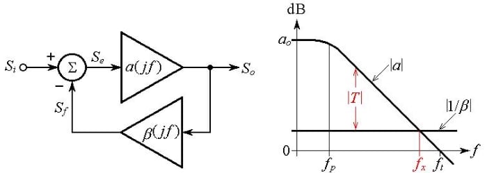
Figure 1. (a) Block diagram of a negative feedback circuit, and (b) visualizing the loop gain T.

This diagram consists of an error amplifier with gain a(jf), a feedback network with transfer function β(jf), and a summing block generating the error signal S_e, 

Equation (1)

Collecting and solving for S_e gives

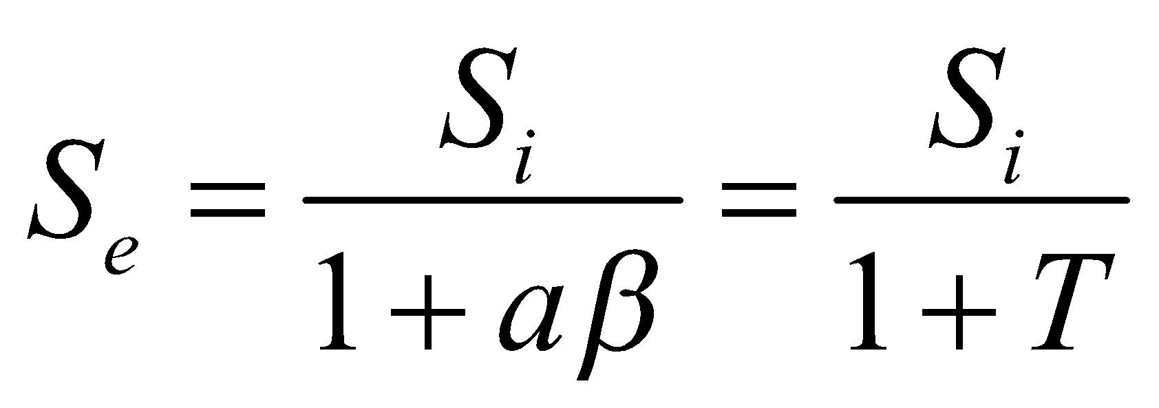
Equation (2)

where T = aβ is called the loop gain because any signal entering the amplifier and going clockwise around the loop, is first amplified by a and then by β, for an overall gain of aβ. It is apparent that larger T leads to smaller S_e for a given input S_i.

Rewriting as T = a/(1/β), taking the logarithms, and multiplying by 20 to convert to decibels, gives

Equation (3)

indicating that we can visualize the decibel plot of |T| as the difference between the decibel plots of |a| and |1/β|. This is depicted in Figure 1b for the case of a constant gain-bandwidth product op-amp and a frequency-independent β.

The frequency f_x at which the two curves intersect, aptly called the crossover frequency, plays an important role in the circuit’s stability (or lack thereof). At this frequency, we have |T(jf_x)|_dB = 0, or |T(jf_x)| = 1. Should the phase ph[T(jf_x)] ever reach –180°, then we’d have T(jf_x) = –1, which, substituted into Eq. (2), indicates that S_e would blow up and lead to oscillation. (Note that even if we set S_i = 0, the intrinsic noise of the circuit would trigger the buildup of S_e.) To prevent oscillation, we must make sure that ph[T(jf_x)] is away from the dreaded value of –180° by a sufficient amount, aptly called the phase margin ɸ_m,

    ɸ_m = 180° + ph[T(jf_x)] 

Equation (4)

Phase margins of practical interest are ɸ_m = 90°, ɸ_m = 65.5° (which marks the onset of peaking in the ac response), ɸ_m = 76.3° (which marks the onset of ringing in the transient response), and ɸ_m = 45° (which we’ll see to lend itself to easy geometric visualization, though it results in a peaking of 2.4 dB and ringing with an overshoot of 23%).

In the situation depicted in Figure 1b, 1/β is a real number, so its phase is 0° and we have ph[T(jf_x)] = ph[a(jf_x)] ≈ –90°, owing to the fact that f_x >> f_p. Consequently, ɸ_m ≈ 180° + (–90°) = 90°. However, things are not always this rosy, so we turn to the more general cases of Figure 2 to estimate the phase margins of the various cases. To this end, we shall use the rate-of-closure (ROC).

What Is Rate of Closure?

Rate of closure or ROC is defined as the difference between the slopes of the ⎪1/β⎪and of the⎪a⎪ curves right at the crossover frequency:

Equation (5)

Once we know the ROC, we estimate the phase margin as

Equation (6)

In Figure 2, we assume an error amplifier with a more general gain profile than the constant gain-bandwidth product type of Figure 1a. (For easy drawing, we are using straight segments, though we know that in practice the sharp angles are rounded, as the |a| curve in Figure 1b.)

(a)

(b)

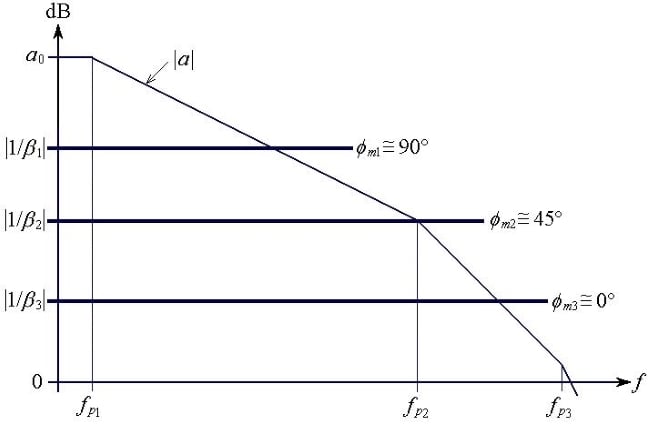
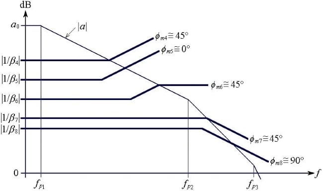
Figure 2. (a) Frequently encountered phase-margin situations with (a) frequency-independent and (b) frequency-dependent feedback factor β(jf).

Now, past the first pole frequency f_p1, ⎪a⎪ rolls off at a rate of –20 dB/dec, and past the second pole frequency f_p2 it rolls off at a rate of –40 dB/dec. Right at f_p2 the slope must be the mean of the two slopes, or –30 dB/dec. Likewise, past f_p3, ⎪a⎪ rolls off at a rate of –60 dB/dec, and the slope right at f_p3 must be –50 dB/dec.

• In Figure 2a the ⎪1/β₁⎪ curve has a slope of 0 and intercepts the⎪a⎪ curve in the region where ⎪a⎪ rolls off at a rate of –20 dB/dec, so Eq. (5) gives ROC = 0 –(–20) = 20 dB/dec, and Eq. (6) gives ɸ_m1 ≈ 180 – 4.5×20 = 90°.
• The ⎪1/β₂⎪ curve has a slope of 0 and intercepts the⎪a⎪ curve at f_p2, where the⎪a⎪ curve has a slope of –30 dB/dec, so Eqs. (5) and (6) give ROC = 0 –(–30) = 30 dB/dec, and ɸ_m2 ≈ 180 – 4.5×30 = 45°.
• The ⎪1/β₃⎪ curve has a slope of 0 and intercepts the⎪a⎪ curve in the region where ⎪a⎪ has a slope of –40 dB/dec, so Eqs. (5) and (6) give ROC = 0 –(–40) = 40 dB/dec, and ɸ_m3 ≈ 180 – 4.5×40 = 0°.
• In Figure 2b the slope of the ⎪1/β₄⎪ curve changes from 0 dB/dec below its crossover frequency to +20 dB/dec above its crossover frequency, so right at the crossover its slope must be +10 dB/dec. Then, Eqs. (5) and (6) give ROC = +10 –(–20) = 30 dB/dec, and ɸ_m4 ≈ 180 – 4.5×30 = 45°.
• The slope of the ⎪1/β₅⎪ curve at its crossover frequency is +20 dB/dec, so Eqs. (5) and (6) give ROC = +20 –(–20) = 40 dB/dec, and ɸ_m5 ≈ 180 – 4.5×40 = 0°.
• The slope of the ⎪1/β₆⎪ curve changes from +20 dB/dec immediately below its crossover frequency to 0 dB/dec above its crossover frequency, so right at the crossover its slope must be +10 dB/dec. Then Eqs. (5) and (6) give ROC = +10 –(–20) = 30 dB/dec, and ɸ_m6 ≈ 180 – 4.5×30 = 45°.
• The slope of the ⎪1/β₇⎪ curve changes from 0 below its crossover frequency to –20 dB/dec above its crossover frequency, so right at the crossover its slope must be +10 dB/dec. Moreover, the slope of the⎪a⎪ curve is –40 dB/dec, so Eqs. (5) and (6) give ROC = –10 –(–40) = 30 dB/dec, and ɸ_m7 ≈ 180 – 4.5×30 = 45°.
• The slope of the ⎪1/β₈⎪ curve at its crossover frequency is –20 dB/dec, and that of the⎪a⎪ curve is –40 dB/dec, so Eqs. (5) and (6) give ROC = –20 –(–40) = 20 dB/dec, and ɸ_m8 ≈ 180 – 4.5×20 = 90°. It is interesting that even though crossover occurs in the region where ⎪a⎪ rolls off at the steep rate of –40 dB/dec, just like the ⎪1/β₃⎪ curve does, the –20 dB/dec slope of the ⎪1/β₈⎪ curve ameliorates the phase margin dramatically compared to the ⎪1/β₃⎪ case.

It pays to regard ROC as the angle between the ⎪1/β⎪and ⎪a⎪curves at the point where they intersect. As this angle becomes narrower, the circuit becomes more stable. Conversely, the wider this angle is, the closer the circuit is to instability.

The phase-margin estimate provided by the ROC method can be fairly good if all pole and zero frequencies are at least a decade away from the crossover frequency. Even if this is not the case, the ROC method still provides a reasonable starting point. After gaining enough experience, a designer will be able to figure out an improved estimate for the phase margin.

A Real-Life Example of Rate-of-Closure

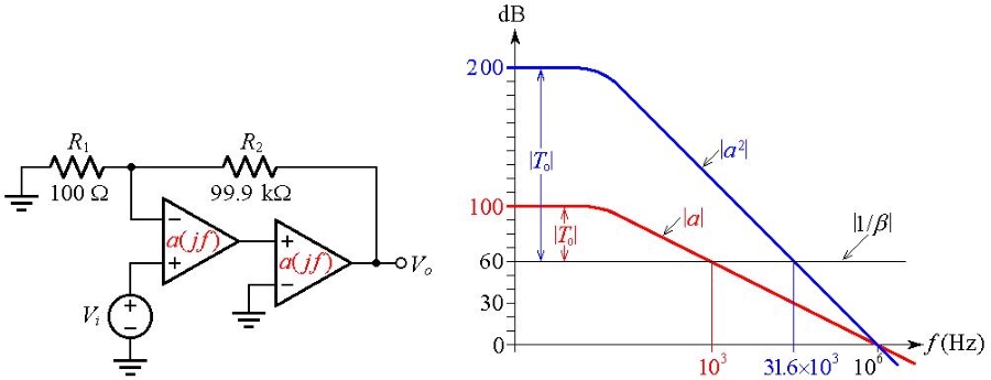
Let us apply the above considerations to a real-life example. Suppose we want to design a high-precision amplifier with (a) a DC closed-loop gain of 10³ V/V (or 60 dB), and (b) a DC loop gain T₀ of at least 10⁶. All we have at hand are op amps having a DC gain of 10⁵ V/V (or 100 dB) and a 1 MHz constant gain-bandwidth product (i.e., a transition frequency of f_t = 1 MHz).

After drawing the ⎪a⎪ and ⎪1/β⎪ curves as in Figure 3b, we note that with a single op-amp we’d have a stable circuit (its situation is similar to the⎪ 1/β1⎪ case of Figure 2a), but with T₀ = 100 – 60 = 40 dB, or 10², which is insufficient. To jazz up T₀ let’s use two op-amps in cascade, for an overall gain of a×a = a². Now we do meet the T₀ requirement (T₀ = 200 – 60 = 140 dB, or 10⁷ >10⁶), but the slope of |a²| at the crossover frequency is –40 dB/dec, indicating that we are in the situation of the ⎪1/β₃⎪ case of Figure 2a, with ɸ_m ≈ 0°. We need to stabilize the circuit by suitably

(a)                                                                                                                       (b)

Figure 3. (a) Composite amplifier intended for a DC closed-loop gain of 60 dB with a DC loop gain T₀ ≥ 10⁶. (b) Bode diagram showing that the composite has ɸ_m ≈ 0° and thus needs frequency compensation. Click to enlarge.

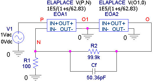
Figure 4. PSpice circuit to simulate the amplifier of Figure 3a.

modifying its ⎪1/β⎪ curve in the vicinity of the crossover frequency f_x, which in our example can be seen to be the geometric mean of 1 kHz and 1 MHz, or f_x = (10³×10⁶)^1/2 = 31.6 kHz. The ⎪1/β₇⎪ case of Figure 2b suggests that for ɸ_m ≈ 45° we need to bend the curve downwards by establishing a breakpoint right at f_x, a task that we accomplish by placing a capacitor C_f in parallel with R₂ and imposing the condition

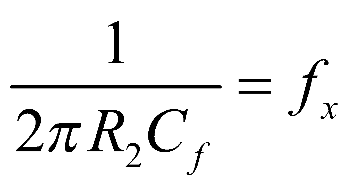
Equation (7)

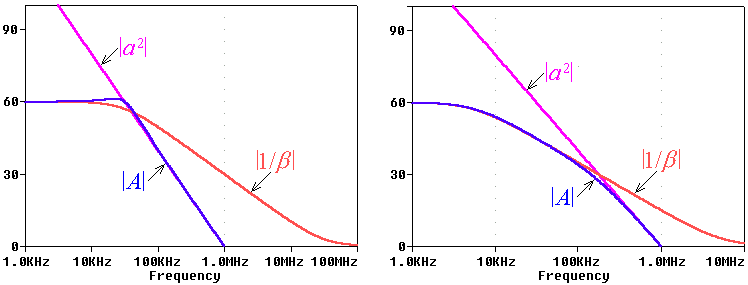
Plugging in f_x = 31.6 kHz and R₂ = 99.9 kΩ gives C_f = 50.36 pF. Running the PSpice circuit of Figure 4, we get the traces of Figure 5a, where we measure f_x ≈ 40.2 kHz and ɸ_m ≈ 51.6°. The ac response A = V_o/V_i exhibits some peaking, and the transient response (not shown but easily verifiable) exhibits some ringing.

(a)                                                                                                       (b)

Figure 5. Plots of |a²|, ⎪1/β⎪, and the closed-loop gain |A| for (a) C_f = 50.36 pF, and (b) C_f = 283.3 pF.

To avoid peaking and ringing, let’s establish a situation of the type of the ⎪1/β₈⎪ case of Figure 2b. We achieve this by shifting our ⎪1/β⎪ curve leftwards until it intercepts the |a²| curve at the point where |a²| drops to 30 dB, or 31.6. This occurs at a new crossover frequency of f_x = (31.6×10³×10⁶)^1/2 = 178 kHz. To find the new breakpoint f₀ of the ⎪1/β⎪ curve, we exploit the constancy of the gain-bandwidth product on the slanted portion of the ⎪1/β⎪ curve and impose 31.6×178×10³ = 10³×f₀. This gives f₀ = 5.623 kHz, so we now need C_f = 1/(2π × 99.9 × 10³ × 5.623 × 10³) = 283.3 pF.

Rerunning the PSpice circuit of Figure 4, but with this new value of C_f, we get the plots of Figure 5b, where we measure f_x ≈ 177.8 kHz and ɸ_m ≈ 86.4°. We got rid of peaking and ringing, but at the price of a lower closed-loop bandwidth of about 5.8 kHz.

Conclusion

This article has presented a graphical, frequency-domain method that provides a straightforward way to assess the stability of a negative-feedback system. By examining the intersection of the curves representing the open-loop gain and the inverse of the feedback factor β, we can determine the rate of closure, and from the rate of closure we can calculate an approximate phase margin.

As you’re reviewing this material, give particular attention to Fig. 2, because most circuits encountered in practice conform to one of the cases depicted in the figure, at least in the proximity of the crossover frequency.