Simulating Current-Pump Performance with Tolerance and Temperature

Last week, I wrote a pair of articles about a constant-current-source circuit that consists of two op-amps and five resistors:

 

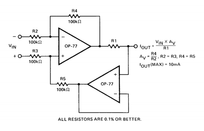
Diagram of a precision current pump. Image used courtesy of Analog Devices

 

In the second of these two articles, I used LTspice to assess the influence of imperfect resistor matching on the circuit’s error, where error was calculated as the difference between the simulated load current and the load current predicted by the formula given in the app note.

 

\[I_{OUT}=\frac{V_{IN}\left(\frac{R4}{R2}\right)}{R1}\]

 

Imperfect matching was simulated by using LTspice’s Monte Carlo function to vary the values of R3 and R5 within a specified tolerance. The magnitude of the output current is directly proportional to the values of R1, R2, and R4, and these three resistors remained at their nominal value.

In this article, we’ll perform a more comprehensive simulation of real-life versus theoretical performance. All of the resistors will have 0.1% tolerance, and we will also incorporate variation in operating temperature. The objective here is to actually understand how much precision we can expect from this circuit under real-life conditions.

 

Simulating at Specific Temperatures

Some of the op-amp components included in LTspice exhibit variations in response to temperature, and some do not. If there is a convenient way to determine which are which, I haven’t been able to find it, so I just used the guess-and-check method.

The LT1001A, which we used in the previous simulation, is not in the temperature-dependency category. After testing a few other op-amps that didn’t fit the bill, I found that the AD8606, which is a precision op-amp intended for low-voltage applications, has temperature dependency somewhere in its macromodel.

We can incorporate temperature into LTspice’s circuit calculations by means of the “temp” directive. For example, “.temp -40 125” will perform a simulation at –40°C and another one at +125°C.

The following circuit indicates whether an op-amp produces different results at different temperatures.

 

   

 

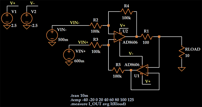
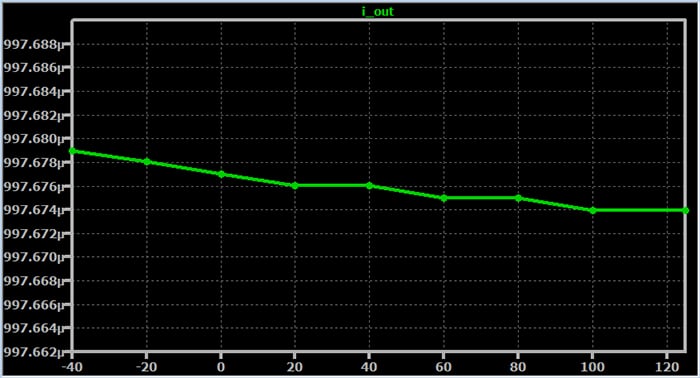
The expected output current is (0.6 V – 0.5 V)/(100 Ω) = 1 mA. Here are the simulated output-current values obtained at the temperatures specified in the “temp” directive:

 

 

Monte Carlo Simulation with Temperature Changes

When we apply the Monte Carlo function (“mc” in LTspice) to the value of a resistor and use the “.step param run ...” directive, the simulation will consist of multiple independent runs, and for each run, the mc function will select a new value from within the range determined by the specified tolerance.

We’ll pretend that the intended application requires functionality over the entire automotive temperature range, which is –40°C to +125°C. This also happens to be the operating temperature range of the AD8606. If we add a “temp” directive, the number of runs will be multiplied by the number of temperatures in the list.

Including numerous temperatures within the range would lead to long simulation times, and it’s difficult to imagine a scenario in which that would be necessary. An op-amp isn’t going to exhibit severe fluctuations in performance in response to a moderate increase or decrease in operating temperature.

In fact, the previous plot indicates that the effect of temperature is monotonic and very subtle. Thus, I think we can adequately account for temperature influences by selecting several temperatures that cover the entire range.

Here’s the schematic that I used for the resistor-tolerance-plus-temperature simulation:

 

 

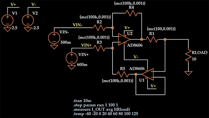
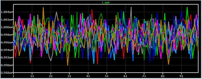
And here is a plot of the simulated load current for the 900 runs (100 runs per temperature).

 

 

Performance Statistics

My preferred next step is to export the results as a text file and then import the text file into Excel for further analysis. To do this, right-click on the plot and select File -> Export data as text. This is what the data look like after I import the text file into Excel:

 

 

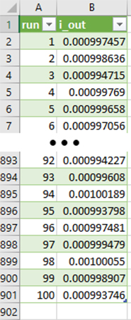
Now I can easily calculate whatever statistics I’m interested in. The average value is 0.9977 mA, so some non-ideality in the op-amp created a small offset (0.0023 mA, or 0.23% of the expected output current). The standard deviation is 2.86 µA, and the maximum and minimum values are 1.0053 mA and 0.9899 mA.

I find the maximum and minimum results quite impressive: even with all resistors subject to 0.1% tolerance and temperature varying over a wide interval, I can expect the load current to not deviate from the desired current by more than about 5 µA in the positive direction and 10 µA in the negative direction.

 

Conclusion

We’ve combined a Monte Carlo method with LTspice’s “temp” directive to explore the realistic performance of a two-op-amp precision current source. Statistical analysis of the simulation results indicates that the circuit offers excellent precision over a very wide temperature range.