LTspice Performance Analysis of a Precision Current Pump

The previous article introduced a circuit that I am referring to as the two-op-amp current source (or current pump).

Here’s the schematic:

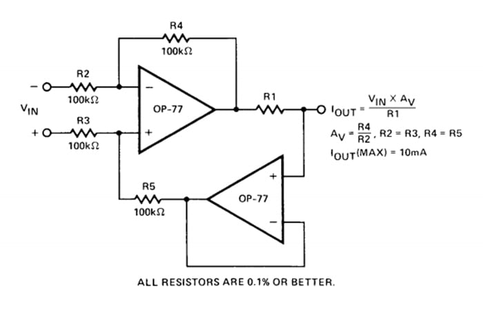
Diagram of a precision current pump. Image used courtesy of Analog Devices

I presented an LTspice implementation of this topology, and we looked at the results of a basic simulation. However, I would like to know more about this circuit, especially since it is described as a precision current pump. What kind of precision can we really expect from this circuit?

In this article, we’ll perform simulations intended to answer three questions. 

1. How precise is the output current under ideal conditions?
2. How is the precision of the output current influenced by load variations?
3. What is the typical and worst-case precision when resistor tolerances are taken into account?

Baseline Precision

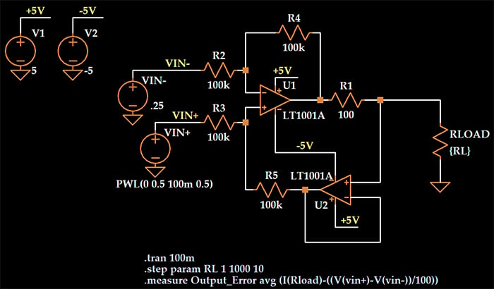
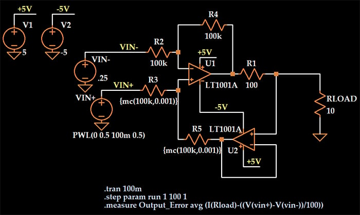
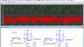
This is the circuit that we’ll use for the first simulation:

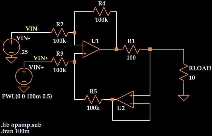
The voltage applied to the differential input stage changes from –250 mV to 250 mV during a 100 ms interval. The formula that relates input voltage to output current tells us that the current flowing through the load should be V_IN/100.

To see how closely the generated load current matches the theoretical prediction, we will plot the difference between the simulated load current and the mathematically calculated load current.

The error is extremely small, and its magnitude varies in proportion to the magnitude of the load current.

Load Regulation

When we’re talking about a voltage regulator, load regulation refers to the regulator’s ability to maintain a constant voltage despite variations in load resistance. We can apply this same concept to a current source: How well does the circuit maintain the specified output current for different values of R_LOAD?

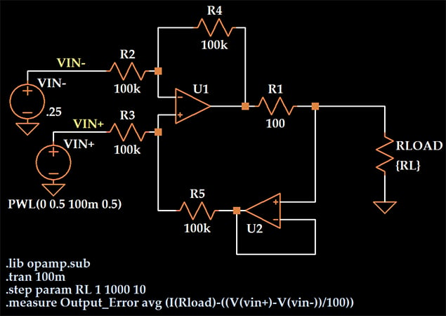
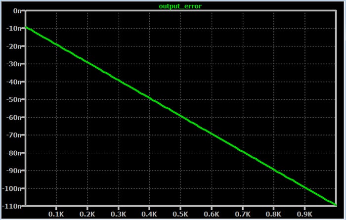
For this simulation, we’ll provide a fixed input voltage of 250 mV, and we’ll use a “step” directive to vary the load from 1 Ω to 1000 Ω in 10 Ω steps.

A “measure” directive allows us to plot error versus the stepped parameter (i.e., the load resistance) rather than versus time; this is accomplished by opening the error log (View -> SPICE Error Log), right-clicking, and selecting “Plot .step’ed .meas data.”

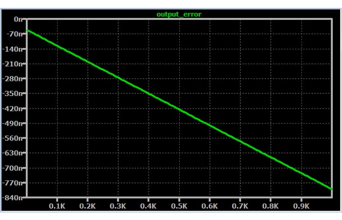
For larger load resistances, the output-current error does increase significantly—from about 50 nA to 800 nA. However, 800 nA is still a very small error.

How much do you think the load regulation will change if we replace the ideal op-amp with a macromodel intended to approximate the performance of a real op-amp? Let’s take a look.

The percentage of variation in output error is quite similar. In the first simulation, the error increased by a factor of 15.7 over the range of load resistance. In the second simulation, where I used the macromodel for the LT1001A, it increased by a factor of 12.1.

What’s interesting is that the LT1001A performed better than the LTspice “ideal single-pole operational amplifier”—the magnitude of the error was much lower over the entire range, and the error was more stable relative to load resistance. I’m not sure how to explain that. Maybe the ideal single-pole op-amp isn’t as ideal as I thought.

The Effect of Resistor Tolerances

We don’t need simulations to determine the effect of variations in the resistance of R1; the mathematical relationship between input voltage and output current gives us a clear idea of how much error will be introduced by an R1 value that deviates from the nominal value.

Also, the circuit diagram taken from the app note indicates how the ratio of R4 to R2 will affect output current, since this ratio determines A_V, and I_OUT is directly proportional to V_IN multiplied by A_V.

Less clear, however, is the effect of imperfect matching between resistors. The circuit diagram indicates that R2 and R3 should be matched and that R4 and R5 should be matched. We can investigate this by performing a Monte Carlo simulation in which resistor values are varied within their tolerance range.

If the simulation includes a large number of Monte Carlo runs, the maximum and minimum errors reported in the simulation results can be interpreted as the worst-case error associated with resistor tolerance.

For this simulation, we will leave R2 and R4 fixed at 100 kΩ; this prevents variations in A_V. We will degrade the circuit’s matching by applying the Monte Carlo function to the values of R3 and R5.

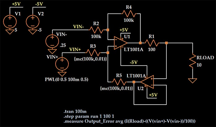
As indicated by the “step” SPICE directive, one simulation consists of 100 runs. The value “mc(100k,0.01)” specifies a nominal resistance of 100 kΩ with a tolerance of 1%.

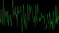
Here is a plot of output-current error for the 100 runs.

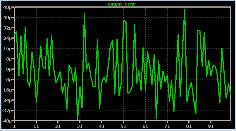
The average error is 15.6 µA, which is 0.6% of the expected 2.5 mA output current, and under worst-case conditions, the actual output current deviates from the expected current by approximately 40 µA.

I’d call that very good precision. Let’s see how the situation improves when we use 0.1% tolerance instead of 1%.

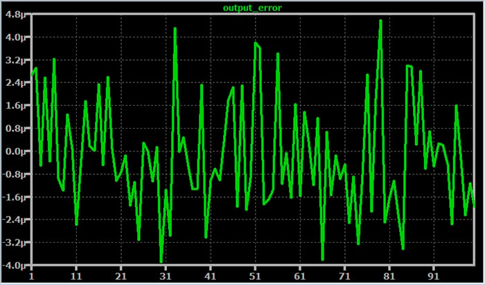
Now the average error is 1.6 µA, which is only 0.06% of the expected output current, and the worst-case error has decreased into the 4 µA range.

Conclusion

We’ve carried out LTspice simulations that have provided valuable insight into the performance of the two-op-amp current pump.

Resistive tolerance of 1%, with the resistors that determine input gain fixed at their theoretical value, allows for high precision. A tolerance of 0.1% applied to all resistors would provide good performance, and since 0.1% resistors are readily available and not expensive, I agree with the author of the app note when he recommends 0.1% tolerance rather than 1% tolerance.