Transferring SPICE Models From LTspice to QSPICE

In the first article of this series, we created and briefly analyzed an LED blinker circuit in LTspice. In the second article, we transferred the circuit to QSPICE using a combination of netlist copy-paste and manual schematic entry. However, the LED in the LTspice circuit (Figure 1) wasn’t available in the QSPICE library.

Figure 1. The LED blinker circuit we created in LTspice.

As a workaround, I replaced the LED with a normal silicon diode in series with a voltage supply (V_FWD). The resulting schematic is shown in Figure 2.

Figure 2. A QSPICE LED blinker circuit based on the LTspice schematic in Figure 1. Note the LED implementation.

The forward voltage of the LTspice LED was 1.83 V. By adjusting the value of V_FWD accordingly, I can conveniently approximate the current-voltage behavior of the original LED model. In this case, “convenient” is what I was looking for and “approximate” is all we really need.

I could also have solved the LED problem by importing the missing model from LTspice. Though this method takes a bit more time and effort, it’s probably the one you’ll end up using in your own designs. We’ll go through this process step by step in the next section.

The SPICE Model Approach

The first step of this process is to find the SPICE model description for the component you used in LTspice. In this case, we used a diode with part number QTLP690C. Go to the “lib” folder in the LTspice directory, open the “cmp” folder, and then open the file “standard.dio” in a text editor. Once the file is open, you can search for the relevant part number (Figure 3).

Figure 3. The .model statement for the QTLP690C diode as it appears in the “standard.dio” text file.

Copy the .model statement to your clipboard and paste it into the QSPICE schematic editor. As shown in Figure 4, QSPICE will ask you if you want to automatically incorporate that SPICE behavior into a schematic symbol. Click YES, place the symbol, and you’re done.

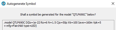
Figure 4. When you paste in the .model statement, QSPICE will ask you about automatically generating a symbol.

With the QTLP690C LED component added, our schematic looks like Figure 5.

Figure 5. A new schematic for our QSPICE LED blinker circuit that incorporates the imported SPICE model.

Now for the disappointing part: this schematic is nonfunctional. The LED blinker is a finicky circuit, and somewhere deep in the SPICE calculations there is enough difference between the LTspice and QSPICE circuits to prevent oscillation. Don’t despair, though, because all we need to do is add a little bit of extra forward voltage to the LED. The added voltage is circled in red in Figure 6.

Figure 6. To make the new schematic work, we need to add a bit of forward voltage.

To summarize, the SPICE model approach consists of nine steps:

1. Go to the “lib” folder in the LTspice directory.
2. Open the “cmp” folder.
3. Open the file “standard.dio” in a text editor
4. Locate the relevant part number within the file.
5. Copy the .model statement to your clipboard.
6. Paste the .model statement into the QSPICE schematic editor.
7. Click YES when prompted to “Autogenerate Symbol.”
8. Place the symbol in the schematic.
9. Tweak as necessary.

We now have two versions of the LED blinker circuit ready for us to run simulations.

Transient Simulation and Basic Plot Analysis in QSPICE

The schematics in Figure 2 and Figure 5 both include a .tran statement specifying a 10 second transient simulation. To run the simulation, press F5. Our goal is to examine the LED’s illumination behavior, so we’ll click on the diode component to plot the current flowing through it.

Figure 7 shows the current waveforms produced by the circuit with the workaround diode (in green) and the circuit with the imported SPICE model (in red).

Figure 7. LED current waveforms for both versions of the QSPICE blinker circuit.

Figure 8 zooms in on a period when the LED is illuminated.

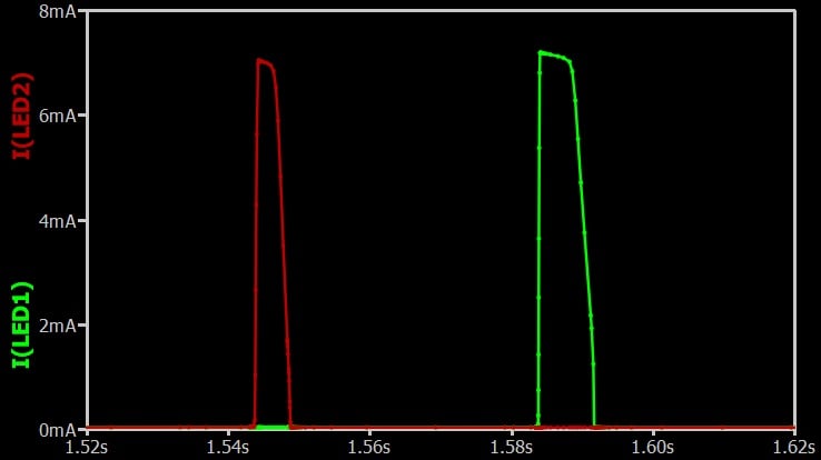
Figure 8. Current through the LED of the workaround circuit (green trace) and the SPICE model circuit (red trace) when the LED is illuminated.

Let’s analyze these results. We’ll start by using waveform cursors to determine the pulse frequency for the LED workaround circuit. Double-click on the I_LED1 trace to activate the first cursor, then double-click again to activate the second cursor. As shown in Figure 9, the frequency information will appear underneath the plot.

Figure 9. Double-click a trace to activate the cursor.

We can see in Figure 9 that the pulse frequency of the LED workaround circuit is 2.55 Hz. To find the same information for the imported-SPICE-model circuit, we simply repeat the process described above for I_LED2 rather than I_LED1. Though I chose not to reproduce the graph here, the pulse frequency for the latter circuit is 4.1 Hz. Note that you can easily grab and move the cursors by clicking on the red cursor-position rectangles.

The cursors also help us to compare pulse widths, as we see in Figures 10 and 11.

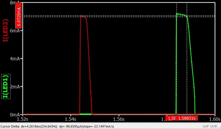
Figure 10. Pulse width for the workaround circuit.

Once again, the information we’re looking for is underneath the graph. The pulse width is 4.26 ms for the workaround circuit…

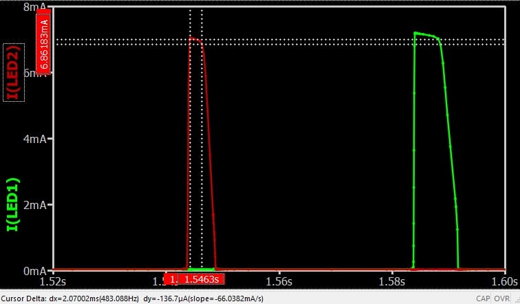
Figure 11. Pulse width for the SPICE model circuit.

…And 2.1 ms for the circuit with the imported SPICE model.

As you may have noticed, the QSPICE cursor interface is very different from the LTspice cursor interface. In keeping with QSPICE’s avoidance of dialogue boxes, the LTspice cursor window has been replaced with cursor data that appears within the plot window itself. Individual cursor positions are displayed along the horizontal and vertical axes; information related to the difference between cursor positions is displayed below the graph.

Key Takeaways

Though the pulse width and oscillation frequency for the two versions of the blinker circuit are different, the differences aren’t extreme. Both versions are useful for simulations, and neither is incorrect—the QTLP690C was selected simply to get the original LTspice simulation started, and a physical circuit would need some trial-and-error adjustments anyway.

Still, the differences actually are useful to our discussion. They'll lead us to some important insights about the electrical behavior in the next article, which will be the last one in this series. We'll also explore some operational details of the imported-SPICE-model version of the LED blinker circuit.

This article is Part 3 of a series on QSPICE for LTspice users. Below is a complete list of articles in this series:

1. Introduction to QSPICE for LTspice Users
2. Transferring LTspice Schematics to QSPICE
3. Transferring SPICE Models from LTspice to QSPICE
4. Using QSPICE to Understand and Tune an LED Blinker Circuit

Featured image used courtesy of Adobe Stock; all other images used courtesy of Robert Keim