Understanding Memory: How to Use Structures in Embedded C Language

How do processors access memory? Learn more about structures in C language and how to use them.

This article will first explain the memory access granularity concept so that we can develop a basic understanding of how a processor accesses memory. Then, we’ll take a closer look at the concept of data alignment and investigate the memory layout for some example structures.

In a previous article on structures in embedded C, we observed that rearranging the order of the members in a structure can change the amount of memory required to store a structure. We also saw that a compiler has certain constraints when allocating memory for the members of a structure. These constraints referred to as data alignment requirements, allow the processor to access variables more efficiently at the cost of some wasted space (known as “padding”) that may appear in the memory layout.

This article will first explain the memory access granularity concept so that we can develop a basic understanding of how a processor accesses memory. Then, we’ll take a closer look at the concept of data alignment and investigate the memory layout for some example structures.

It’s worthwhile to mention that the memory system of a computer can be much more complicated than what’s presented here. The goal of this article is to discuss some basic concepts that can be helpful when programming an embedded system.

 

Memory Access Granularity

We usually envision memory as a collection of single-byte storage locations as shown in Figure 1. Each of these locations has a unique address that allows us to access the data of that address.

 

Figure 1

 

However, a processor usually accesses memory in chunks larger than one byte. For example, a processor may access memory in four-byte chunks. In this case, we can envision the 12 consecutive bytes of Figure 1 as shown in Figure 2 below.

 

Figure 2

 

You may wonder what the difference is between these two ways of handling memory. With Figure 1, the processor reads from and writes to memory one byte at a time. Note that, before reading a memory location or writing to it, we need to access that cell of memory, and each memory access takes some time. Assume that we want to read the first eight bytes of the memory in Figure 1. For each byte, the processor needs to access the memory and read it. Hence, to read the content of the first eight bytes, the processor will have to access the memory eight times.

With Figure 2, the processor reads from and writes to memory four bytes at a time. Hence, to read the first four bytes, the processor accesses address 0 of memory and reads the four consecutive storage locations (address 0 to 3). Similarly, to read the next four-byte chunk, the processor needs to access memory one more time. It goes to address 4 and reads the storage locations from address 4 to 7 simultaneously. With byte-sized chunks, eight memory accesses are required to read the eight consecutive bytes of memory. However, with Figure 2, only two memory accesses are required. As mentioned above, each memory access takes some time. Since the memory configuration shown in Figure 2 reduces the number of accesses, it can lead to greater processing efficiency.

The data size that a processor uses when accessing memory is called the memory access granularity. Figure 2 depicts a system with four-byte memory access granularity.

Memory Access Boundary

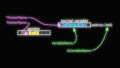
There’s another important technique that hardware designers often employ to make a processing system more efficient: they restrict the processor such that it can access memory only at certain boundaries. For example, a processor may be able to access the memory of Figure 2 only at four-byte boundaries, as depicted by the red arrows in Figure 3.

 

Figure 3

 

Is this boundary limitation going to make the system significantly more efficient? Let’s take a closer look. Assume that we need to read the content of the memory locations with address 3 and 4 (indicated by the green and blue rectangles in Figure 3). If the processor could read a four-byte chunk starting from an arbitrary address, we could access address 3 and read the two desired memory locations with a single memory access. However, as mentioned above, the processor cannot access an arbitrary address directly; rather, it accesses the memory only at certain boundaries. So how is the processor going to read the content of address 3 and 4 if it can access only the four-byte boundaries?

Due to the memory access boundary limitation, the processor has to access the memory location with address 0 and read the four consecutive bytes (addresses 0 to 3). Next, it has to use shift operations to separate the content of address 3 from the other three bytes (addresses 0 to 2). Similarly, the processor can access address 4 and read another four-byte chunk from address 4 to 7. Finally, shift operations can be used to separate the desired byte (the blue rectangle) from the other three bytes.

If there were no memory access boundary limitation, we could read addresses 3 and 4 with a single memory access. However, the boundary limitation forces the processor to access the memory twice. So why do we need to restrict memory access to certain boundaries if it makes data manipulation more difficult? Memory-access boundary limitation exists because making certain assumptions about the address can simplify the hardware design. For example, assume that 32 bits are required to address all the bytes within a block of memory. If we limit the address to four-byte boundaries, then the two least significant bits of the 32-bit address will always be zero (because the address will always be evenly divisible by four). Hence, we’ll be able to use 30 bits to address a memory with 2³² bytes.

Data Alignment

Now that we know how a basic processor accesses memory, we can discuss data alignment requirements. Generally, any K-byte C data type must have an address that is a multiple of K. For example, a four-byte data type can be stored only at addresses 0, 4, 8, …; it cannot be stored at addresses 1, 2, 3, 5, …. Such restrictions simplify the design of the interface hardware between the processor and the memory system.

As an example, consider a processor with four-byte memory access granularity that can access the memory only at four-byte boundaries. Assume that a four-byte variable is stored at address 1, as shown in Figure 4 (the four bytes correspond to the four different colors). In this case, we’ll need two memory accesses and some extra work to read the unaligned four-byte data (by “unaligned” I mean that it is split across two four-byte blocks). The procedure is shown in the figure.

 

Figure 4

 

However, if we store a four-byte variable at any address that is a multiple of 4, we’ll need only a single memory access to modify the data or read it.

That’s why storing K-byte data types at an address that’s a multiple of K can make the system more efficient. Hence, C language “char” variables (which require only one byte) can be stored at any byte address, but a two-byte variable must be stored at even addresses. Four-byte types must start at addresses that are evenly divisible by 4, and eight-byte data types must be stored at addresses evenly divisible by 8. For example, assume that on a particular machine, “short” variables require two bytes, “int” and “float” types take four bytes, and “long”, “double”, and pointers occupy eight bytes. Each of these data types should normally have an address that’s a multiple of K, where K is given by the following table.

 

Data Type	K
char	1
short	2
int, float	4
long, double, char*	8

 

Note that the size of different data types can vary depending on the compiler and the machine architecture. The sizeof() operator would be the best way to find the actual size of a data type.

Memory Layout for a Structure

Now, let’s examine the memory layout for a structure. Consider compiling the following structure for a 32-bit machine:

struct Test2{

	uint8_t	    c;
        uint32_t    d;
        uint8_t	    e;
	uint16_t    f;

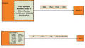
} MyStruct;

We know that four memory locations will be allocated to store the members within the structure, and the order of memory locations will match that of declaring the members. The first member is a one-byte variable and can be stored at any address. Hence, the first available storage location will be allocated to this variable. Assume that, as shown in Figure 5, the compiler allocates address 0 to this variable. The next member is a four-byte data type and can be stored only at addresses that are a multiple of 4. The first available storage location is address 4. However, this requires leaving addresses 1, 2, and 3 unused. As you can see, the data alignment requirement leads to some wasted space (or padding) in the memory layout.

The next member is e, which is a one-byte variable. The first available storage location (address 8 in Figure 5) can be allocated to this variable. Next, we reach f, which is a two-byte variable. It can be stored at an address that’s divisible by 2. The first available space is address 10. As you can see, more padding will appear in order to satisfy the data alignment requirements.

 

Figure 5

 

We expected the structure to occupy 8 bytes, but it actually requires 12 bytes. Interestingly, if we are aware of the data alignment requirements, we may be able to rearrange the order of the members within a structure and make memory usage more efficient. For example, let’s rewrite the above structure as given below, where the members are ordered from the largest one to the smallest.

struct Test2 {
    
     uint32_t       d;
     uint16_t       f;
     uint8_t        c;
     uint8_t        e;
    
} MyStruct;

On a 32-bit machine, the memory layout for the above structure will probably look like the layout depicted in Figure 6.

 

Figure 6

 

Whereas the first structure required 12 bytes, the new arrangement requires only 8 bytes. This is a significant improvement, especially in the context of memory-constrained embedded processors.

Also, note that there can be some padding bytes after the last member of a structure. The total size of a structure must be divisible by the size of its largest member. Consider the following structure:

struct Test3 {
    
        uint32_t     c;
        uint8_t      d;
    	    
} MyStruct2;

In this case, the memory layout will be as shown in Figure 7. As you can see, three padding bytes are added to the end of the memory layout to increase the size of the structure to 8 bytes. This will make the structure size divisible by the size of the larger member within the structure (the c member, which is a four-byte variable).

 

Figure 7

 

Summary

• A processor usually accesses memory in chunks larger than one byte. This can increase system efficiency.
• The data size that is used when a processor accesses memory is the processor’s memory access granularity.
• A processor may be restricted to accessing memory only at certain boundaries (e.g., at four-byte boundaries).
• This memory-access limitation exists because making certain assumptions about the address can simplify the hardware design.
• Generally, any K-byte C data type must have an address that is a multiple of K. Such restrictions simplify the design of the interface hardware between the processor and the memory system.
• The data alignment requirement leads to some wasted space (or padding) in the memory layout.
• There can be some padding bytes after the last member of a structure. The total size of a structure must be divisible by the size of its largest member.

To see a complete list of my articles, please visit this page.