
How to Obtain the Temperature Value from a Thermistor Measurement
This article explains how to use an NTC or a PTC thermistor with an ADC, along with the various process techniques to convert ADC measured results into a usable temperature value.
All of the products that I have designed in my career have had some form of temperature circuit in them. The simplest and most cost-effective circuits use a negative temperature coefficient (NTC) or positive temperature coefficient (PTC) thermistor to measure temperature. The most basic circuit is based on a resistor divider attached to a low-cost microcontroller (MCU) with an analog-to-digital converter (ADC). This article explains how to use an NTC or a PTC thermistor with an ADC, along with the various process techniques to convert ADC measured results into a usable temperature value.
Voltage from the Thermistor
A typical thermistor circuit provides a voltage (VSense) that is applied to an ADC input; the ADC then converts this voltage to an LSB (least significant bit) digital value that is proportional to the input voltage. A common ADC resolution is 12 bits for many low-cost MCUs, so the formulas in this article will use 12-bit resolution. Figure 1 shows both the voltage-divider and constant-current circuits.
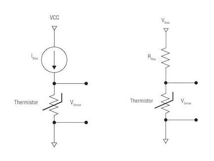
Figure 1. Voltage-divider and constant-current circuit implementations
You can use Equation 1 to convert the measured 12-bit ADC LSB value to a voltage:
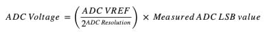
where the ADC resolution (12-bit ADC (212)) is 4,096 total bits, VREF is 3.3 V and the measured ADC LSB value is 2,024 (example ADC LSB value from a Texas Instruments (TI) TMP61 thermistor family test board).
For example:
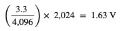
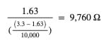
Equation 2 calculates the resistance from the voltage divider’s VSense:
For example:
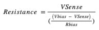
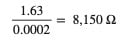
Equation 3 calculates the resistance from the constant current, Ibias:
where Ibias is 200 µA (default standard current for a TMP61 family part) and VSense is 1.63 V.
For example:
Conversion Methods
Once you have converted the voltage to an ADC representation, there are a number of ways to get the actual temperature from the thermistor’s VSense voltage. The most common method uses a look-up table (LUT), also known as a resistance table, normally provided by the thermistor manufacturer. A 1°C LUT table has 166 elements and must be stored in your controller, but this uses up controller memory. To reduce the number of elements, you could use a 5°C LUT, but then you may have some linear error in the calculation. A 5°C LUT will require 33 elements, but no one wants to see 5°C resolution, so further processing of the LUT will be necessary in order to get better than 5°C or 1°C of resolution. I will discuss this further in the Linear Interpolation section.
Another method is to use a Steinhart-Hart equation, which is based on a 3rd order polynomial curve fit. It will require natural log math to complete, and you must have a floating-point controller or floating-point math libraries to perform the calculations. The Steinhart-Hart equation is more accurate than a LUT.
PTCs can use a polynomial equation, given the linear output of the device. Polynomial equations are the most accurate way to get a temperature from a thermistor. A polynomial is a mathematical expression of variables that involves only the operations of addition, subtraction, multiplication and non-negative integers. Another way to describe polynomials is that they provide a curve-fit equation for a slope. You must apply the polynomial fit yourself and then solve the regression function (the temperature based on the curve fit) to obtain the temperature. Most PTCs are based on polynomials.
Don’t be concerned; once you get the hang of polynomials, you will get better accuracy; plus, you will not need a LUT in your controller. These are simple math functions that can process faster than an LUT with interpolation. TI has a design tool that can provide you with a LUT or fourth-order polynomial and regression function, with examples of how to apply these math functions in C code for your controller to get the most accurate temperatures from a thermistor.
Look-up Tables
A LUT typically ranges from -40°C to 125°C, but will vary based on the thermal limits of the thermistor. There are two types of LUTs: the 1°C and 5°C. See Figure 2 for examples.
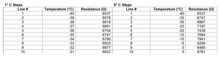
Figure 2. 1°C and 5°C table examples for the TMP61 thermistor family
The LUT method works like this:
- Store the 1°C step LUT into your controller’s memory.
- Calculate the measured resistance value based on the read ADC LSB value.
- Find the closest match of resistance in the stored LUT. The corresponding temperature to that found resistance value will be the resulting temperature.
- If you want greater accuracy instead of rounding to the nearest value in the LUT, you will need to do a linear interpolation of the 1°C step LUT. Using the 5°C step LUT saves some memory space because it is a smaller table and interpolation will provide reasonable accuracy. There will be a small linear step error in the temperature calculation, however.
Linear interpolation
Interpolation is calculating and inserting an intermediate value that was derived between two known values.
The interpolation method works like this:
- Store a 1°C or 5°C step LUT into your MCU’s memory.
- Calculate the measured resistance value based on the read ADC LSB value.
- Calculate how far the measured resistance is from the two closest resistance values in the LUT. Apply that same ratio of the corresponding resistance to the temperature values (also known as a linear approximation of the actual temperature between two points).
Equation 4 is the formula for the linear interpolation process:
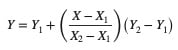
Where X is the known value of thermistor resistance, Y is the unknown value of temperature, X1 and Y1 are the closest values lower than the known resistance for resistance and its associated temperature, and X2 and Y2 are the closest values higher than the known resistance for resistance and its associated temperature.
The Y value will be the closest temperature value between the upper- and lower-temperature values on your LUT.
If the LUT is provided in 5°C steps, be aware that converting it to a 1°C LUT using linear interpolation can have a linear error of 0.5°C. This is a mathematical error from calculating between two values in linear steps. A 1°C LUT is usually best if you can get it from the manufacturer.
Steinhart-Hart Equation
The Steinhart-Hart equation is a 3rd order polynomial using natural logs. It can be an accurate method to derive temperature from a known resistance. The equations used in the Steinhart-Hart method need three resistance values from the thermistor’s LUT to calculate the estimated curve fit:
- R1 = resistance at the lowest temperature (T1 = -40°C).
- R2 = resistance at a middle temperature (T2 = 25°C).
- R3 = resistance at the highest temperature (T3 = 125°C).
You can use these variables in the coefficient formulas below, and you only need to calculate once.
You must resolve each of these elements in order to determine the three coefficients needed to calculate the Steinhart-Hart equation, where ln is a natural log.
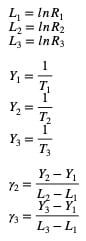
Formulas 5, 6, and 7 will provide the coefficients needed to calculate the temperature; you only need to calculate once.
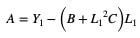
Equation 8 calculates the temperature. You will use Equation 8 every time you want to know the temperature from the calculated resistance.
Where *T is the temperature in Kelvin (°C = °K - 272.15) (°F = (1.8 × °C) + 32).
Polynomials
3rd and 4th order polynomials are the most accurate and fastest way to calculate the temperature values for TI's thermistor portfolio; you will not need a LUT. The quartic function is a 4th order polynomial that results in a resistance value based on a temperature. Using the regression formula will result in a temperature value based on a measured resistance.
Begin by opening a blank spreadsheet in Microsoft Excel. Input the temperature and resistance values from the LUT of your device. Plot the typical resistance, as shown in Figure 3, using a scatter plot, not a line plot.
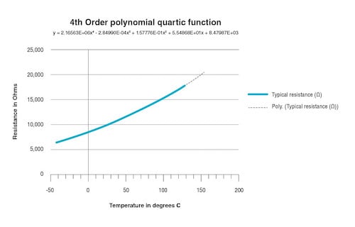
Figure 3. Quartic function plot
With temperature on the X axis and resistance on the Y axis, right-click the plot line and select “Add Trend Line”. Figure 4 shows the format trendline window. Select “Polynomial” and change the order to “4.

Figure 4. Trendline in Excel
At the bottom of the Format Trendline window, select “Display Equation on Chart” and “Display R Squared Value on Chart.” The displayed equation in the plot will be your 4th order polynomial quartic function, enabling you to get the resistance value from the temperature. An alternate method to get the coefficients is to use Excel’s LINEST function; the syntax is LINEST(known_y's, [known_x's], [const], [stats]). Remember that a 4th order polynomial has five coefficients.
In the trendline-provided 4th order polynomial, you will notice some numbers use addition and some use subtraction. The quartic function below uses all addition. In the coefficients, change the sign of the coefficient to negative in order to subtract according to the trendline polynomial.
A 4th order polynomial is a quartic function and is calculated in formula 9 where resistance is a function of temperature.
R(Ω) = A4*(T4) + A3*(T3) + A2*(T2) + A1*T + A0
Where R is the resistance of the thermistor, T is the temperature and A0/A4 are coefficients.
| Coefficients | |
| 8.479874E+03 | A0 |
| 5.548683E+01 | A1 |
| 1.577759E-01 | A2 |
| -2.849901E-04 | A3 |
| 2.165629E-06 | A4 |
Regression Function
A regression function is the reverse of a 4th order polynomial. Simply swap the X axis for the Y axis, as shown in Figure 5. The 4th order polynomial equation shown in the plot will use the resistance value to find the temperature.
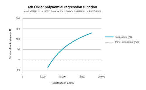
Figure 5. Regression plot
The 4th order polynomial regression in formula 9 with temperature as a function of resistance: (Y = Y axis which is the temperature)
T°C = A4*(R4) + A3*(R3) + A2*(R2) + A1*R + A0)
Where R is the resistance of the thermistor, T is the temperature and A0/A4 are coefficients listed in Figure 5.
Accuracies
R2 is the fit value of the trendline for the polynomial curve. An R² = 1.00000E+00 is a perfect fit and the error is minimal in calculating the resistance from the polynomial. Acceptable R2 values are R2 = 0.999 and below.
Tolerances for temperature accuracies will vary depending on your application. A 1%-3%°C accuracy will work for most temperature measurement applications. I always recommend determining this value at the beginning of your design and attempting to meet this goal.
Potential Errors
Most errors in calculating temperature using formulas result from mathematical and rounding errors. Figure 6 provides an example of mathematical errors caused by rounding. A good practice to remember is that the more digits beyond the decimal point that you use (such as 0.123456), the more accurate the formula will be.
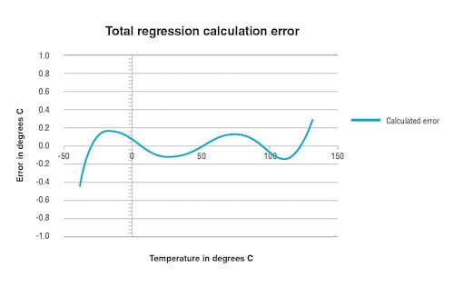
Figure 6. Regression errors
I recommend using at least six digits – preferably nine or 12 digits beyond the decimal point – for better accuracies. The optimal number of digits beyond the decimal point is 16. Although this is possible and easy for a spreadsheet, it’s not always practical for an MCU. Six digits will provide better than 0.4°C accuracies across the entire temperature range, which is still more accurate than a LUT. The regression calculation plot in Figure 6 shows the potential error with six digits beyond the decimal point.
Conclusion
As you can see, there are multiple ways to process an ADC LSB value obtained after converting a measured voltage coming from a thermistor voltage divider circuit. The simplest methods are not necessarily the most accurate, but may be just fine for your application. Most of these methods will work for both NTC and PTC devices.
I would rank the methods from best to adequate as:
- Fourth-order polynomial (linear feedback devices only)
- Third-order polynomial (linear feedback devices only)
- Steinhart-Hart equation
- 1°C LUT with interpolation
- 5°C LUT with interpolation
- 1°C LUT
- 5°C LUT
Achieving real accuracy is a system-wide design effort. The Vbias resistor in a resistor-divider circuit, the tolerance of your thermistor, the VCC error, the VREF error, ADC errors, calculation methods, and mathematical errors all add up to the final accuracy.
To learn more, visit TI’s linear thermistor portfolio.
Industry Articles are a form of content that allows industry partners to share useful news, messages, and technology with All About Circuits readers in a way editorial content is not well suited to. All Industry Articles are subject to strict editorial guidelines with the intention of offering readers useful news, technical expertise, or stories. The viewpoints and opinions expressed in Industry Articles are those of the partner and not necessarily those of All About Circuits or its writers.


