Facebook
 Google
 GitHub
 Linkedin
How to Analyze Data from a Custom PCB Sensor Subsystem
A quick walkthrough of how to analyze data from a custom precision sensor system.
Learn a method for analyzing data from a custom precision sensor system, translating sensor data into usable noise measurement information.
I recently designed a high-precision inclinometer subsystem that is so sensitive to environmental forces that it needed a custom housing on a granite slab to function correctly.
Throughout the design process, I have laid out my BOM, schematic, PCB layout, housing design, and firmware. I've also gone through a test and measurement phase to characterize the noise the board generates.
My final step in this process is to analyze the data that I can gather from my subsystem. This article looks at the data captured off of the board and shows how I chose to visualize the data.
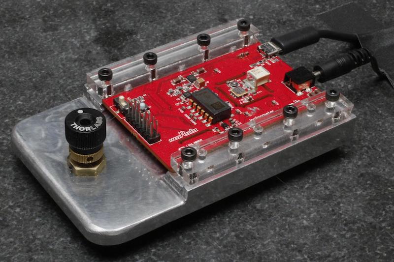
The finished custom PCB
If you'd like to learn more about the rest of the project, please check out the links below:
- How to Design a Precise Inclinometer on a Custom PCB (full project overview)
- Schematic Design
- PCB Layout
- Firmware Design
- Noise Characterization
Data Analysis
The LTC2380IDE-24, the successive approximation register (SAR) analog-to-digital converter (ADC) I chose to use in my design, has integrated data averaging that is easy to implement. Conversion results are held in internal memory and combined with previous results until an SPI transaction occurs.
To average two results, toggle the CNV pin to logic high twice before reading the data out. To average 65,535 results, toggle the CNV pin 65,535 times before reading the data out.
The data the sensor produces is 40 bits long: 24 bits for the sensor reading and 16 bits to indicate how many samples were averaged (note that the count is indexed at 0—i.e., a value of 0 indicates that 1 sample was averaged, a value of 1 indicates that 2 samples were averaged, and so forth). If you look at the data file attached at the end of this document, you will notice that I added an additional 16 bits to the data to track the measurement number (these numbers were not used in the analysis).
I transferred the data off the PCB as sequences of ASCII ‘0’ and ‘1’ and processed it on the computer with Mathematica. The first 24 bits were converted to decimal notation and multiplied by a scale factor of $$\frac{15°}{2^{23}}%0$$. The next 16 bits were converted to a decimal number and appear in parentheses in the left side of the footer of each graphic below as the number of repeated measurements. Each trial consisted of 1023 samples, and each sample consisted of n averaged readings (1,2,4,8,...,32768).
All trials were performed consecutively in a single run with no significant pause between measurements.
Each trial is presented with the same set of graphics and calculations. Mean and standard deviation are calculated for the raw data and used to create a probability density function. Raw data is grouped in bins and also displayed in a histogram. A scatterplot shows the data points after processing through an n-tap moving average (FIR) filter. Finally, colored triangles are used to indicate the maximum, mean + standard deviation, mean, mean - standard deviation, and minimum data points at three different scales (100%, 1%, 0.01%).
We’ll first take a look at the data and then discuss the significance of the results.
_resize.gif)
As you’ll recall from statistics class, the mean is the simple average of all measurements. Standard deviation provides an indication of spread. For our purposes, we would like the standard deviation to be as small as possible.
You’ll see the mean remains constant throughout processing, with any variation easily attributed to rounding error (as expected.) The standard deviation (SD), which indicates the spread of the data, decreases as the number of FIR taps increases -- this is due to the fact that the moving average filter is mitigating the effects of outlying data points. I also show the standard deviation of the data after it has been put through an averaging filter to allow interested readers to compare the effects of averaging inside the ADC (digital averaging filter) with averaging outside the ADC (moving average filter).
The mean of this dataset is 0.6987°, with no smoothing or data manipulation, and the standard deviation is 0.0025°. That provides a standard deviation that is 3 orders of magnitude lower than the mean. The standard error is even smaller at 0.000078°. But do all of these decimal places really matter? That’s a phenomenally small standard deviation. A 6 standard deviation range (6σ) is 0.015° -- giving me a 99.999999% probability that a single value I read off of my device is within 0.015° of the actual value. It’s possible that the device is capable of even greater resolution, but my experimental setup or PCB design introduces too much noise.
Now -- for the next question. Can I do better? Statistically, I can collect more measurements. However, if I don’t want to sit around and wait for the device to collect thousands of data points, and use a large amount of processor memory and processor power, what would be an acceptable device configuration? For that, let’s look at another experiment—consisting of the same 1023 trials of 32768 average readings. If I stored 32768 32-bit measurements inside the microcontroller, I’d need at least 131 kB of memory and who knows how many clock cycles to process the accumulated data. If I want to average 32768 measurements inside the ADC, I simply toggle the Convert pin 32768 times.
Using the digital averaging filter inside the ADC shifts the burden of storage and computation away from the microcontroller—freeing it up to do other things.
.gif)
Here, 32768 trials are averaged inside the ADC -- providing an average of 0.701° with a standard deviation of 0.000547°. A 6σ range is 0.003° and there is a 99.999999% chance that a single measurement is between 0.688° and 0.704°.
Conclusion
Perhaps my inclinometer wasn’t quite as precise as I wanted it to be, but the fact is that I created a subsystem that offers more precision than I’ll ever need: I can measure an inclination down to one hundredth of a degree and know that the difference between the measured value and the actual value is negligible. At this point I have no plans to build, adjust, or characterize anything that would need more precision than that.
Do you have any projects or systems that could benefit from a high-precision inclinometer design such as this one? Is there a feature or capability that you would like to see added to this subsystem? Feel free to share your thoughts in the comments section below.
All datasets shown below:
.gif)
.gif)
.gif)
.gif)
.gif)
.gif)
.gif)
.gif)
.gif)
.gif)
.gif)
.gif)
.gif)