
More on Noise-Canceling Headphones: Adaptive Controllers in Active Noise Control Systems
Active noise control is a principle technology in noise-canceling headphones. But there's a nuanced part of the ANC conversation that warrants discussion: adaptive controllers and cancelation paths.
With more people working from home, noise-canceling headphones are becoming increasingly popular. In a previous article, we discussed that active noise control (ANC) requires an adaptive algorithm to adjust the filter coefficients and optimize noise attenuation. This is due to the fact that the noise characteristics as well as the system response can vary with time.
This article, which builds on essential concepts on ANC from the first article, will assess the adaptive controller of an ANC system in greater detail.
Gradient Descent Algorithm
An ANC system attempts to find optimum filter weights by minimizing the mean square value of the sound that is picked up by the error microphone.
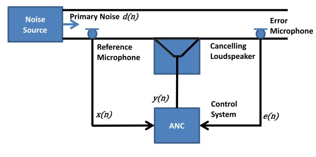
Duct-acoustic feedforward ANC system. Image used courtesy of Alina Mirza
The mean square value of error, referred to as error surface in the rest of the article, is a multivariable function of the filter coefficients. For example, with a two-tap filter, the error surface is a bowl-like function as depicted below:
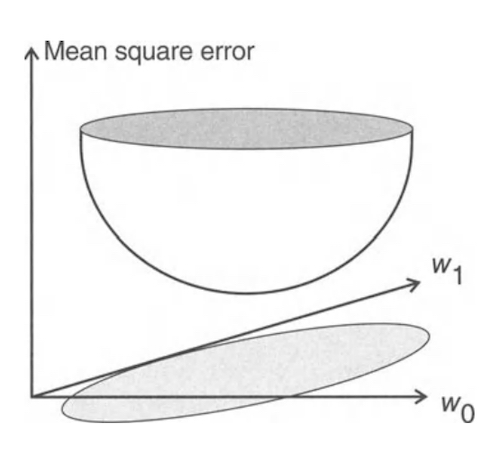
Image courtesy of Scott D. Snyder
The adaptive algorithm should find the filter weights corresponding to the bottom of this bowl. A commonly-used technique to achieve this is a gradient descent algorithm. This optimization algorithm starts with an initial guess of the optimum filter weights and updates them iteratively to find the optimum values.
The algorithm calculates the partial derivative (or gradient) of the error surface with respect to a filter weight to decide how the initial value of that weight should be updated. You can better understand this mechanism by considering a single-variable error function such as f(x)= x2 as depicted below:
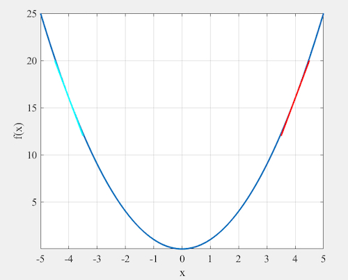
The minimum of this error function occurs at x=0. If our current location is x=4, the derivative of f(x) (which is the same as the slope of the red line) is a positive value. In this case, we should decrease the current value to decrease f(x). However, with a current weight value of x=-4, the derivative of f(x) is negative (the slope of the cyan line).
In this case, we should increase x to decrease f(x). Hence, whether we should increase or decrease x can be determined by the derivative of f(x). This can be extended to a multivariable function; we only need to replace derivative with partial derivative. In the context of the gradient descent algorithm, this partial derivative of the multivariable function is referred to as a gradient.
Based on this discussion, we can use the following equation to iteratively update the weights:
wi, new = wi, old – μ x (partial derivative of the error surface w.r.t wi)
Here, μ is the convergence coefficient and specifies the percentage of the negative of the gradient that is added to the current weight value in each iteration.
The Cancelation Path
In an ANC system, the output of the adaptive filter is converted to an analog signal and then to a sound wave at the output of the loudspeaker. This sound wave goes through the acoustic path between the loudspeaker and the error microphone. Then, it is picked up by the error microphone and converted to a digital signal.
The adaptive algorithm actually receives this digital signal as an input. The path from the output of the digital filter to the input of the adaptive algorithm is usually referred to as the "cancelation path."
If we model the cancelation path by a transfer function S(z), we can model the ANC system by the following block diagram:
.jpg)
Image courtesy of Sen M. Kuo
Summarizing, the error signal for the LMS algorithm is derived from the output of the adaptive filter modified by S(z). This is in contrast to what we have in other common adaptive filter applications. Knowledge of S(z) is required to calculate the gradient for the optimization algorithm. Besides, published reviews of ANC have shown that the system depicted above will be generally unstable.
This issue can be resolved by placing an estimate of S(z) between the reference signal x(n) and the weight update of the LMS algorithm. This is illustrated below where S(z) represents an estimate of the cancelation path transfer function S(z).
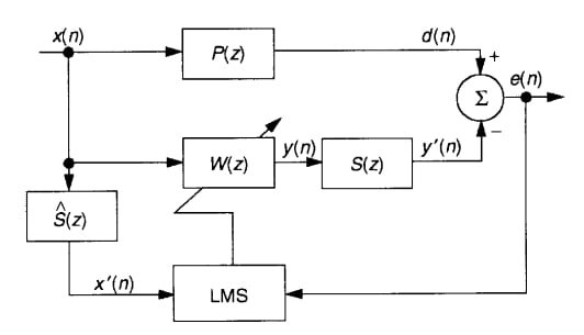
Image courtesy of Sen M. Kuo
Since x(n) is filtered before being applied to the least mean square (LMS) block, this algorithm is called a filtered-X LMS algorithm in the literature.
Cancelation Path Modeling
The cancelation path transfer function S(z) is estimated by employing a second loop of adaptive filtering as shown below.
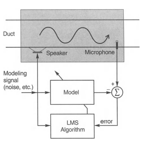
Image courtesy of Scott D. Snyder
An appropriate signal (modeling signal) is applied to both the cancelation path and its “Model.” The “LMS algorithm” monitors the error signal and attempts to minimize it by adjusting the filter weights of the “Model.” When the error signal is minimized, the “Model” response gets closer to that of the cancelation path.
A copy of the obtained model will be used to filter the reference signal of the ANC system as discussed in the previous section. This gives us the following block diagram:

Image courtesy of Colin N. Hansen
Conclusion
These past two articles have reviewed the basics of ANC generally and adaptive controllers in ANC systems specifically. As noise cancelation becomes a staple in more consumer headphone devices, it's likely that more electrical engineers will see how these principles come into play at the circuit level.


