Facebook
 Google
 GitHub
 Linkedin
DC and Steady-state AC Circuit Analysis Made Easy with Python
Learn how utilizing Python and SymPy in DC and steady-state AC circuit analysis can help speed up and simplify calculations like mesh current and phasor current.
Basic electric circuits are linear systems and determining the values of currents or voltages in a circuit requires using linear algebra. I find that when I am “solving” a circuit (i.e., determining the values of the currents flowing through all elements in the circuit), the application of circuit laws is done long before the quantities of interest are determined. In a matter of just a few minutes, we can determine a system of equations that describes the behavior of a simple circuit. However, it might take us quite a while to manually manipulate that set of algebraic equations to find the quantities we are looking for.
Many students and educators often turn to MATLAB for assistance with linear systems such as these, but Python and the SymPy package can also be used to analyze DC and steady-state AC circuits just as easily and for free. Let’s illustrate this by looking at some examples, starting with the DC analysis.
DC Analysis Example—Using Python to Solve Mesh Currents
The circuit in Figure 1 probably doesn’t exist in real life, and it serves no practical purpose.
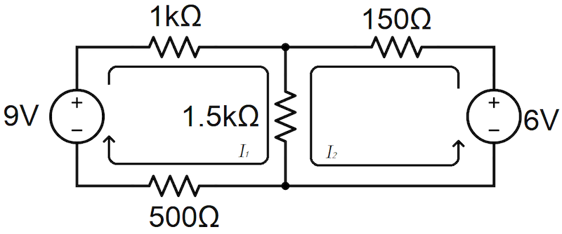
Figure 1. A DC circuit example circuit schematic.
However, in typical circuit analysis textbooks, fully resistive circuits with DC power supplies such as this one are used as a means to practice applying Kirchhoff’s laws and Ohm’s laws in the context of a large circuit.
As a note, I think it helps if you think of these not as circuits that could be real but as puzzles for someone with a particular knowledge base and skill set to solve…for fun!
That aside, I have drawn mesh currents I1 and I2 on this circuit, and we can use the mesh current analysis technique to devise the following Equations 1a and 1b:
$$3kΩ \cdot I_1 + 1.5kΩ \cdot I_2 = 9V$$
Equation 1a
$$1.5kΩ \cdot I_1 + 1.65kΩ \cdot I_2 = 6V$$
Equation 1b
With this system of equations in hand, we are effectively done applying circuit theory. The remaining task of manipulating these equations together to solve for the values of mesh currents I1 and I2 is purely algebraic. Instead of doing so by hand, let’s convert this system of equations to a matrix and use Python to grind through the algebra for us. Our matrix will consist of the resistive coefficients for each mesh current and the voltages on the right-hand side of the equations, as shown in Figure 2.
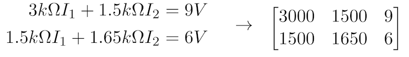
Figure 2. Matrix equations describing the I, R, and V relationships of the circuit of Figure 1.
Next, we turn to Python. I use Google Colaboratory for calculations such as these because it’s web-accessible, and all the libraries I need are available. However, if your Python environment includes the SymPy library, you can use whatever environment you prefer.
To solve our system of equations in Python, let’s first import the SymPy library, then define our matrix, and finally calculate its reduced row echelon form to determine the values of the two mesh currents using the following commands:
from sympy import *
dcEquations = Matrix([[3000, 1500, 9],[1500, 1650, 6]])
dcEquations.rref()
This produces the following output:
(Matrix([
[1, 0, 13/6000],
[0, 1, 1/600]]), (0, 1))
These code snippets tell us that the value for I1 is 13/6000 A, or 2.17 mA, and the value for I2 is 1/600 A, or 1.67 mA.
Steady-state AC Analysis Example Using Python
The method we used to analyze the DC resistive circuit in Figure 1 can also be used to analyze steady-state AC circuits, and it doesn’t take much effort to devise an AC circuit on paper that could actually serve a real purpose. Figure 3 shows a circuit with two reactive loads (inductors), each of which could represent a motor for an air conditioning unit, a sump pump, a refrigerator compressor, or some other household electrical device.
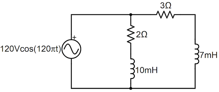
Figure 3. A steady-state AC circuit example with two reactive loads.
The circuit in Figure 3 is called a “steady-state” AC circuit because its power supply has a fixed frequency with constant amplitude. From here, we need to convert the inductances in the circuit to impedances (in units of ohms) so that we can use the mesh current method to analyze its steady-state behavior. Therefore, we calculate impedances for the inductors in the circuit according to Equation 2, using the driving frequency of our source as ω (120π rad/s).
$$Z_L = jωL$$
Equation 2.
In Figure 4, we re-draw the circuit with impedances labeled for each passive element and phasor mesh currents I1 and I2.
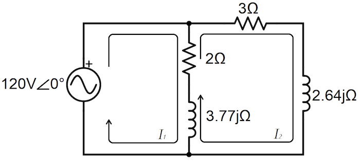
Figure 4. The AC circuit of Figure 3 after converting the inductances to impedances.
Just like we did with the circuit in Figure 1, we can use Kirchhoff’s Voltage Law and Ohm’s Law to derive a system of equations relating the elements and mesh currents in the circuit in Figure 4. Equations 3a and 3b comprise that system.
$$(2 + j3.77)Ω \cdot I_1 − (2 + j3.77)Ω \cdot I_2 = 120V$$
Equations 3a.
$$(2 + j3.77)Ω \cdot I_1 − (5 + j6.41)Ω \cdot I_2 = 0$$
Equation 3b.
Again, the rest of the process used to solve for the mesh currents in the circuit of Figure 4 is pure algebra. The matrix form for this system of equations is shown in Figure 5.
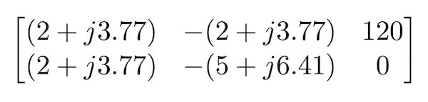
Figure 5. Matrix for Equations 3a and 3b representing the steady-state AC circuit of Figure 4.
The following commands in Python will solve this system of equations for the values of the mesh currents in the circuit in Figure 4. Note that we can use “j” in our matrix definition without any special effort because “j” is defined within SymPy as the imaginary unit in complex space.
from sympy import *
acEquations = Matrix([[2+3.77j,-(2+3.77j), 120],[2+3.77j, -(5+6.41j), 0]])
acEquations.rref()
This produces the following output:
(Matrix([
[1, 0, 35.7203044893402 - 44.6772284258869*I],
[0, 1, 22.5428313796213 - 19.8376916140667*I]]), (0, 1))
This tells us that the phasor currents I1 and I2 are (35.72 – j44.68)A and (22.54 – j19.84)A, respectively. Notice how Python represents the imaginary unit as “I” rather than “j”. To convert these to time-dependent functions, we apply a little bit of trigonometry to find their respective amplitudes and phases. The amplitude and phase of I1 are found through equations 4a and 4b:
$$|I_1| = \sqrt{35.72^2 + 44.68^2} A = 57.20 \space A$$
Equation 4a.
$$θ_1 = atan (\frac{-44.68}{35.72}) = -51.36° = 0.8964 rad$$
Equation 4b.
Similarly, the amplitude and phase of I2 are found according to equations 5a and 5b:
$$|I_2| = \sqrt{22.54^2 + 19.84^2} A = 30.02 \space A$$
Equation 5a.
$$θ_2 = atan({\frac{-19.84}{22.54}}) = -41.35° = 0.7217 rad$$
Equations 5b.
Finally, given those amplitudes and phases, we determine the functional forms for I1 and I2:
$$I_1(t) = (57.20)A \cdot \cos(120πt − 0.8964)$$
Equation 6a.
$$I_2(t) = (30.02)A \cdot \cos(120πt − 0.7217)$$
Equation 6b.
Benefits of Python and SymPy for DC and Steady-state AC Analysis
Note that steady-state AC analysis does require the extra steps of conversion from inductance (and/or capacitance) to complex impedance beforehand and conversion from phasor forms to time-dependent forms afterward. However, applying this matrix technique using Python saves us more computation time when solving AC circuits than DC circuits because Python handles even the complex algebra for us, juggling the added imaginary dimension with ease.
For both DC and steady-state AC circuit analysis, Python and the SymPy library can be easily employed to reduce the amount of work required to determine desired values. While the circuits analyzed in these examples were relatively simple, the technique can scale to more complicated circuits with many more meshes. Using Python in this way not only reduces the amount of time taken to solve circuit problems but it can also help students mentally discriminate between circuit theory and mere algebra as they practice newly-learned network analysis techniques.