 Facebook
 Google
 GitHub
 Linkedin
How Elliptic Curve Cryptography Works
Learn about ECC or elliptic-curve cryptography, including its applications and benefits.
Learn about ECC or elliptic-curve cryptography, including its applications and benefits.
My last article discussed the ingenuity of the Diffie-Hellman key exchange. This article introduces elliptic curves used in a more advanced exchange. (If you'd like a little bit more context, check out my primer on cryptography for some basic information.)
The reason that we use elliptic curves for the key exchange is because they allow longer keys to be generated with fewer bits of data exchanged between computers. This method of cryptography was discovered independently by Neal Koblitz and Victor S. Miller.
Security researchers always knew it was possible to “break” a 512-bit key through brute force, rainbow tables, or some other bit of ingenuity. It was simply thought to take too many computers and too much time.
In the years since the original Diffie-Hellman exchange was first implemented, microprocessors have become faster, smaller, and more affordable. A bad actor today can create a 50-node, 400-core Raspberry Pi computer-cluster for approximately the same cost as a single 8051-based computer from 30 years ago. That means that security researchers and “good guys” need to constantly increase key length to keep the bad guys from figuring out their secrets.
One of the schemes used today is the elliptic-curve Diffie-Hellman exchange.
What Is an Elliptic Curve?
Elliptic curves are a class of curves that satisfy certain mathematical criteria. Specifically, a planar curve is elliptic if it is smooth and takes the commonly used “Weierstrass form” of
$$y^{2}=x^{3}+Ax+B$$
where
$$4A^{3}+27B^{2}≠0$$
You’ll often see these curves depicted as planar slices of what might otherwise be a 3D plot.
On the left, in transparent red, is the 3-dimensional contour plot of y2=x3-3x+z. The orange plane that intersects the 3D contour plot is shown on the right. The curve is “elliptic” everywhere except at the saddle point, where the curve transitions from a closed curve to an open curve.
You might notice that “elliptic curves” do not look like geometric ellipses. That is because “elliptic curves” take their name from a larger class of equations that describe these curves and the ellipses you came to know in school.
$$ay^2+by=cx^3+dx^2+ex+f \quad \{a, b, c ,d, e, f\} \in \rm I\!R$$
The general form of the elliptic curve equation
Elliptic Curve Addition Operations
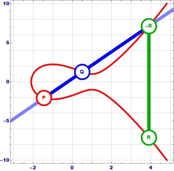
Elliptic curves have a few necessary peculiarities when it comes to addition. Two points on the curve (P, Q) will intercept the curve at a third point on the curve. When that point is reflected across the horizontal axis, it becomes the point (R). So P ⊕ Q = R.
*Note: The character ⊕ is used as a mathematical point addition operator, not the binary XOR operator.
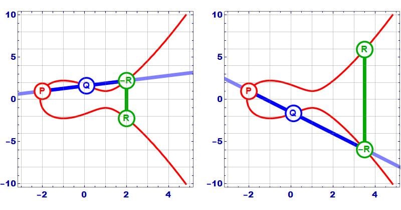
In the graphs above, the two example points P+Q=R.
The line that connects P and Q intersects the curve at a third point, and when that point is reflected across the horizontal axis, it becomes the point R.
This reflection is necessary is for the times where P and Q are at the same point on the curve (P=Q). In those cases, the generated line is tangent to the curve by definition. Without the reflection, it would not be possible to add P to itself multiple times, since P⊕P (2P) would generate the same point as P⊕P⊕P (3P, 4P, nP), etc...
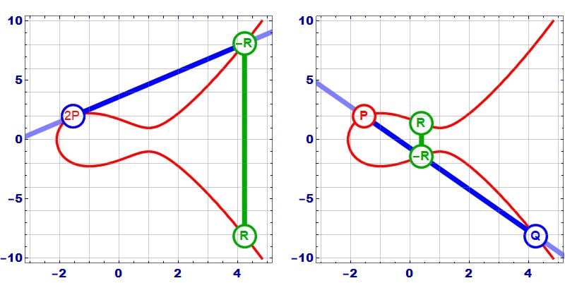
Left: A point that is added to itself (2P) generates a tangent line that intercepts the curve at a new point that when reflected across the horizontal access becomes the point R. Right: Two points (P, Q) that lie on the curve will intercept the curve in a third point, that when reflected across the horizontal access becomes point R.
This, of course, wouldn’t be an ideal mathematical condition. By reflecting below the line, P⊕P=R, and the point P⊕R=P⊕P⊕P=3P ends up generating a new point (-S) somewhere else on the curve. That new point, when added to P, then generates a new point, and so on. Without the reflection, none of this would happen.
The following graphic shows the result of successive addition of P to itself (P⊕P, P⊕2P, P⊕3P, P⊕4P, etc…).
This animation shows the results of P⊕P⊕P⊕P⊕P -- Each frame shows the results of P⊕Q=R (until the animation cycles), with the first frame being P⊕P, and each successive frame using the results of the last frame R to generate the new point Q that is added to the stationary point P. Each point “Q” begins the frame where “R” ended the previous frame (until it recycles at 2P).
The idea behind all of this is that one point on the curve added to itself multiple times will generate other points on the curve. Any two points can be used to identify a third point on the curve. An exception is provided for when P(x,y=0), and the tangent line goes to infinity.
Finding Integer Points on the Curve
To use these curves in cryptography, we have to limit their range, after all, it simply isn’t practical to have numbers near infinity on a 16/32/64-bit microcontroller. So the vertical and horizontal range is capped at a very large prime number, p. The modulus operator is used to keep the results within that range. Then, all integer solutions to the equation that describes the curve are found.
In this example, I’ll use the prime number 281 and the equation
$$y^2=x^3-3x$$
Rearranging and introducing the modulus operator leaves the following equation:
$$(y^2-x^3+3x)(mod\;281)=0$$
In this equation, x and y are integers with values between 0 and 281. When the left side of the equation is computed, divided by 281, and there is no remainder, the point is added to the list below.
Then it is a matter of substituting all integer values of x and y between 0 and 281 into the equation and seeing if the equation is true or not. While the equation can be evaluated by hand, the process is best suited to a computer program.
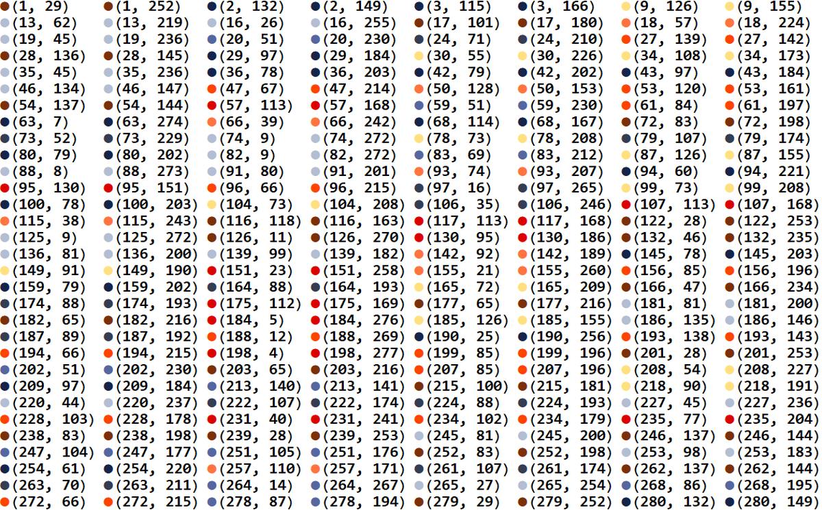
The points that satisfy the equation shown above are color-coded for use in a diagram that is shown below. The colors are based on their y-value distance from 281/2, which is half of the modulus. Note that each x value has only two y values, and the y values are equidistant from the midpoint of the modulus. The colors are introduced simply to aid in pattern recognition in later diagrams
When these points are plotted on cartesian coordinates, certain symmetries become apparent.
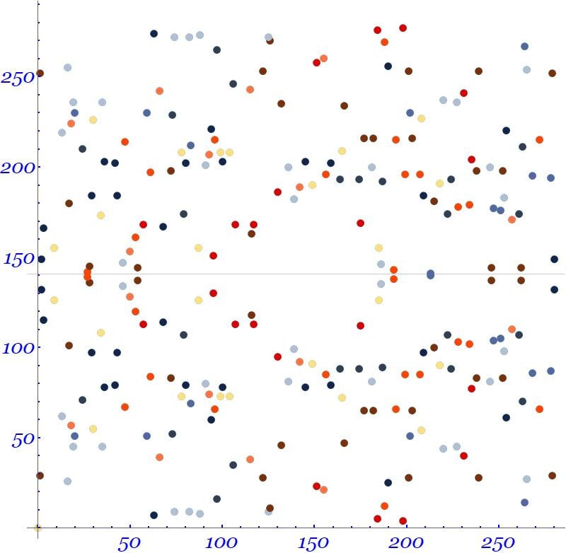
The graph above plots the previously determined points. Note that each x value has two y values that are equally spaced away from the vertical center.
But a planar graph isn’t really the best way to visualize the numbers. When we use the modulus operator, the graph wraps around itself in both the x and y direction once it hits 281; 281 is equivalent to 0, 282 is equivalent to 1, 290 is equivalent to 9, etc. If the graph wrapped in only one direction we could represent it as a cylinder. But it wraps in both and mathematicians tend to imagine those situations with a torus
Datapoints mapped onto the surface of the torus are shown in the following picture, with colored lines provided to help determine orientation.
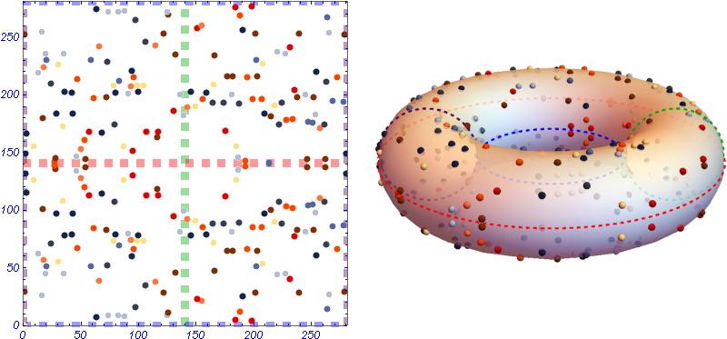
The torus is created such that the vertical midpoint of the graph corresponds to the outer radius of the torus, and the top and bottom of the graph correspond to the inner radius of the torus. In this graphic, the color coding should allow you to see how the points are mapped onto the torus. For example, the clump of points near (50,150) is visible on the near side of the torus on the viewer’s left. Dotted lines are added to assist viewers in determining orientation.
A line of constant slope that travels along the surface of the torus is shown below. This line passes through two randomly selected data-points.
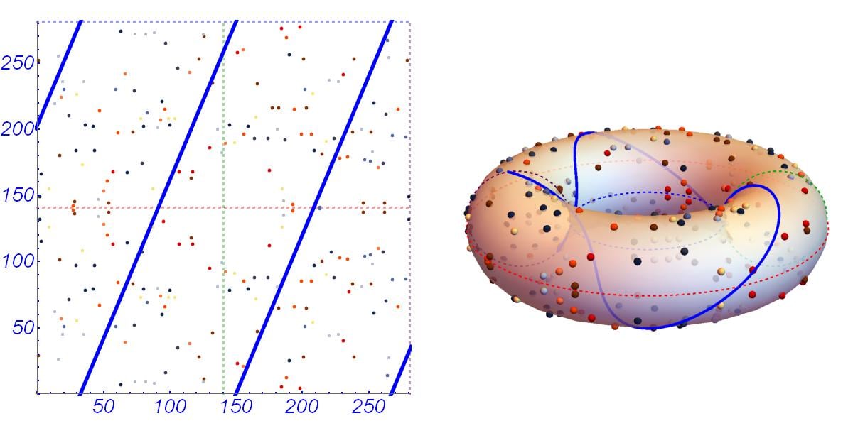
To add two points on the graph, draw a line from the first selected point P = (187, 89) to the second selected point Q = (235, 204), and extend the line until it intersects another point on the graph -R = (272, 215), extending it across the plot boundaries if necessary.
Once you intercept a data-point, reflect the point vertically across the middle of the graph (an orange dotted line that represents y=281/2) to find the new point on the graph (272, 66). Therefore (187, 89) ⊕ (235, 204) = (272, 66)
This is equivalent to what we did earlier. Two points are selected, and a line is drawn between them until it intercepts the third point. Since we calculated the points, we know that they all lie on the graph, and satisfy the equation
$$(y^2-x^3+3x)(mod\;281)=0$$
Putting It All Together—The Diffie-Hellman Elliptic-Curve Key Exchange
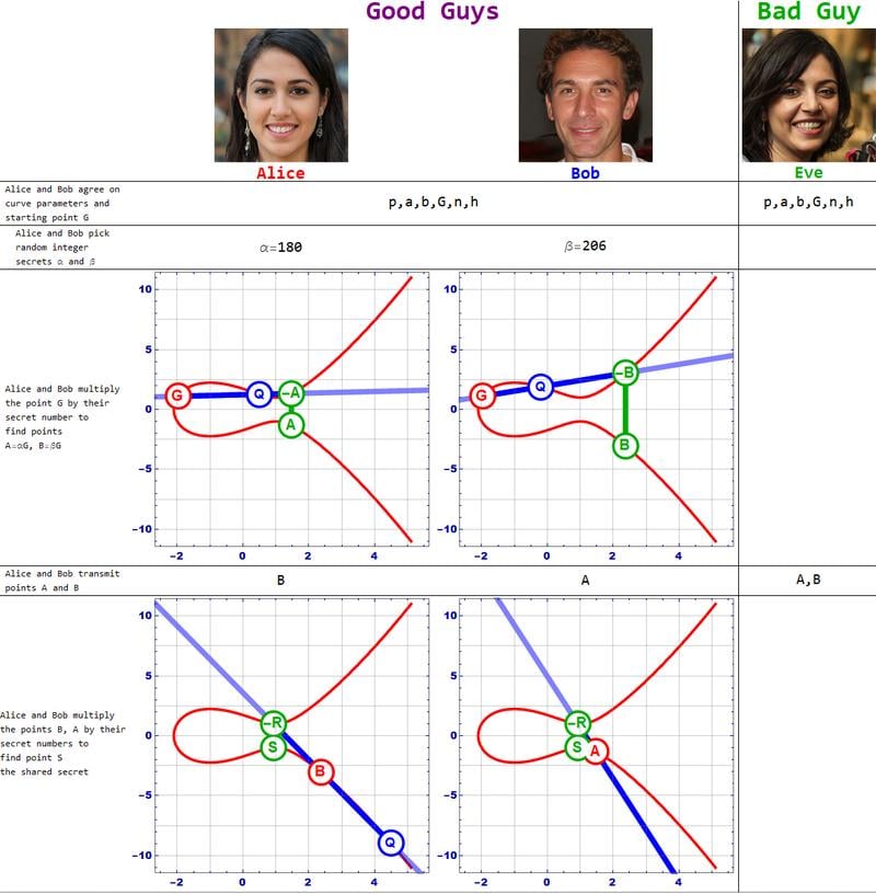
The Diffie-Hellman exchange described in the last article showed how two users could arrive at a shared secret with modular arithmetic. With elliptic-curve cryptography, Alice and Bob can arrive at a shared secret by moving around an elliptic curve.
Alice and Bob first agree to use the same curve and a few other parameters, and then they pick a random point G on the curve.
Both Alice and Bob choose secret numbers (α, β). Alice multiplies the point G by itself α times, and Bob multiplies the point G by itself β times.
In this example, Alice picked α=7 and Bob picked β=5 as their secret numbers.
Each arrive at new points A=αG, and B=βG that they exchange the points with one another.
Starting at the new points, Alice and Bob again multiply their new point by their own secret number.
Bob and Alice multiply their secret number by the point they receive to generate the secret S. This works because, mathematically, S=α(βG)=β(αG).
Once Alice and Bob exchange their public numbers A, and B, they repeat the point computation (αβ) they performed earlier with their until they determine their shared secret S
At the end of the exchange, Bob and Alice have chosen a secret point S on the graph that Eve cannot easily determine.
Remember that we used small numbers to make the process easier to understand. DHEC uses a publicly known equation with large coefficients and modulus, for example, curve1559, which might very well be securing your browser right now.
max: 115792089210356248762697446949407573530086143415290314195533631308867097853951
curve: y² = x³ + ax + b
a=115792089210356248762697446949407573530086143415290314195533631308867097853948
b= 41058363725152142129326129780047268409114441015993725554835256314039467401291
Summary
A great deal of modern cryptography is based upon the Diffie-Hellman exchange, which requires that two parties combine their messages with a shared secret that is difficult for a bad actor to deduce.
Elliptic-curve Diffie-Hellman allows microprocessors to securely determine a shared secret key while making it very difficult for a bad actor to determine that same shared key. The next articles will show how to implement secure communications on a microcontroller project.


Hi there,
I think there might be a small error on the graph where it quotes: “In the graph on the right, the point P(-2.1, 0.2) + the point R (2.9, 4.4) produces the point S(-0.1, -1.8)” (under Elliptic Curve Addition Operations). There is no point S, just P, Q and R.
This article was a really good intro to elliptic curves, thanks!
Hi, the comment near the graph “In the graph on the left, the point P(-2.1, 0.2) plus the point Q(0, -1.7) produces the point R(2.9, 4.4). In the graph on the right, the point P(-2.1, 0.2) + the point Q (2.9, 4.4) produces the point R(-0.1, -1.8)” doesn’t correspond with the picture. For example, the R in the left picture definitely isn’t at coordinates (2.9, 4.4).