Introduction to Pulse Code Modulation (PCM)

In a previous article, we introduced pulse‑amplitude modulation (PAM), where analog samples of the message signal are transmitted at discrete time instants. In other words, PAM is discrete in time but allows the pulse amplitude to vary continuously over its entire range.

A natural next step to consider is making the representation discrete in amplitude as well, leading to what is known as pulse‑code modulation (PCM). In PCM, the sampled values are quantized into a finite set of levels, and each level is encoded digitally.

This article provides an introduction to PCM, describing the core operations of sampling, quantization, and encoding required to generate a PCM waveform. Subsequent articles will delve deeper into each of these stages and discuss the key performance trade-offs in PCM systems.

Definition of PCM and Its Overlap with ADCs

Figure 1 shows the block diagram for generating a PCM waveform.

Figure 1. PCM system diagram.

The lowpass filter preceding the sampling stage is used to prevent aliasing of the message signal. Aliasing refers to the distortion that occurs when a signal contains frequency components higher than half the sampling rate, causing them to “fold back” and appear as erroneous lower frequencies in the sampled signal. This lowpass filter, known as an anti‑aliasing filter, ensures the signal is bandlimited before sampling. Next, the signal undergoes three core operations: sampling, quantization, and encoding. The final PCM output is a serial bit stream that represents the quantized samples in binary form.

If you’re familiar with analog‑to‑digital converter (ADC) concepts, you may have already noticed that the steps involved in generating PCM closely resemble ADC operation. You might wonder what the difference between PCM and analog-to-digital (A/D) conversion is. The similarity between PCM and A/D conversion is strong enough that Leon W. Couch, in Digital and Analog Communication Systems, offers the following definition of PCM:

PCM is essentially analog‑to‑digital conversion of a special type in which the information contained in the instantaneous samples of an analog signal is represented by digital words in a serial bit stream.

With this definition in mind, the key distinction is that PCM explicitly transmits those digital words as a sequence of bits (the PCM stream). In their book Communication Systems, Carlson and Crilly offer the following definition:

PCM is a digital transmission system with an analog-to-digital converter at the input and a digital-to-analog converter (DAC) at the output.

While this definition doesn’t explicitly state that the output is a serial bit stream, it clearly underscores PCM’s strong conceptual link to analog‑to‑digital conversion. To further clarify the difference between these two concepts, note that PCM is a modulation scheme that takes a comprehensive, system‑wide perspective. It presents the theory and format for representing a signal digitally and examines how that representation affects communication system performance, encompassing considerations such as the required transmission bandwidth and system noise behavior.

An ADC, by contrast, is the hardware that performs the sampling, quantization, and encoding operations that PCM relies on. The ADC doesn’t specify how the resulting bits are transmitted, framed, synchronized, or integrated into a communication system. Every PCM system relies on an ADC, and most ADCs internally produce PCM‑compatible outputs. Nevertheless, not every ADC output is used as PCM in a communication system. For example, an ADC in a digital multimeter converts signals for local display and analysis, with no intent to transmit the bits as a serial communication stream. We now examine the three steps necessary for generating a PCM signal: sampling, quantizing, and encoding.

Sampling

The sampling process yields a discrete‑time representation of the message signal. Figure 2 illustrates a 1-Hz sine wave sampled at a rate of f_s = 16 Hz.

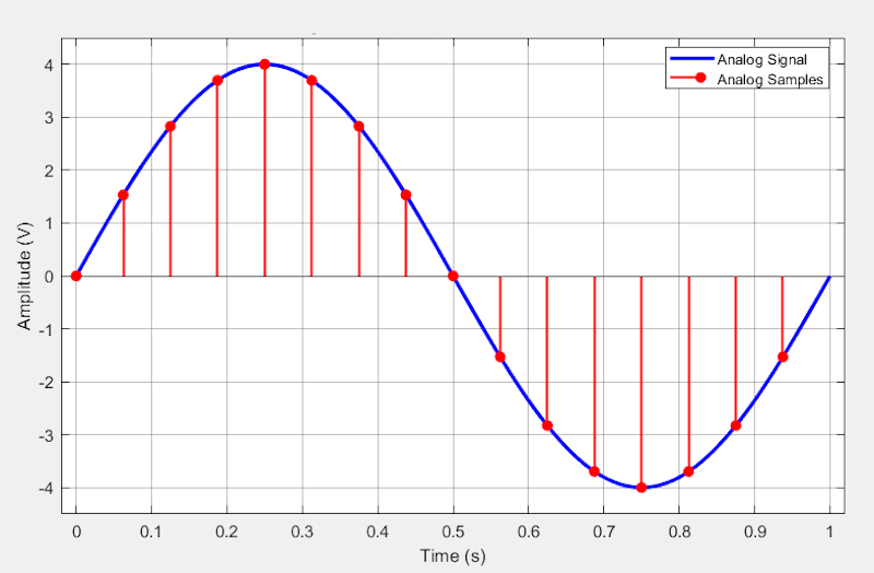
Figure 2. Sampling visualization. The blue curve is the analog input; red stems with circles show the sample times and values.

To maintain fidelity to the original signal, the Nyquist sampling criterion must be fulfilled, which requires the sampling rate to exceed twice the highest frequency component W found in the message signal. To achieve this, a lowpass anti-aliasing filter is employed before the sampler to remove any frequency components above W, as mentioned earlier. The figure above illustrates ideal instantaneous sampling.

In practice, however, sampling circuits hold each discrete value for a fixed duration, creating a sequence of pulses whose amplitudes correspond to the sampled signal values. Therefore, the sampling stage simply produces the flat‑top PAM pulses we examined in the previous article.

Quantization: Uniform Mid-Tread and Mid-Rise Characteristics

The core concept of quantization is straightforward: it generates a discrete-amplitude representation by mapping each sample to the nearest permissible amplitude level. However, the intricacies of the mapping process can differ among techniques. The most commonly used method is uniform quantization, which operates by dividing the analog signal’s amplitude range into L equal-sized intervals. Each sample is then rounded to the midpoint of the interval it occupies. Figure 3 shows the input–output characteristics of two uniform quantizers: the mid‑tread and mid‑rise types.

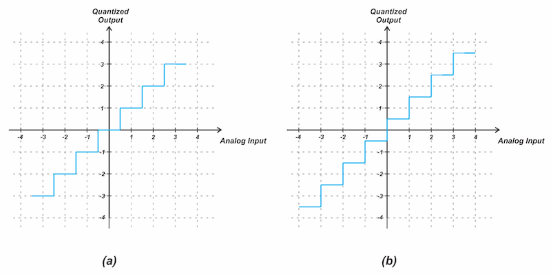
Figure 3. Two types of quantization characteristics: (a) mid-tread and (b) mid-rise.

While a mid‑tread quantizer includes zero as one of its output levels, the mid‑rise quantizer places zero between two quantization levels. How does this affect the system performance? The mid-tread characteristic creates a dead zone in which small‑amplitude inputs collapse to zero. This dead zone helps suppress low‑level noise around zero. In other words, when the input is close to zero and contains small noise, the mid‑tread dead zone forces those fluctuations to zero, creating a stable, noise‑free zero output.

This behavior is particularly useful in speech and audio coding. If a mid‑rise quantizer were used in these applications, small system noise would cause the output to fluctuate between the two levels adjacent to zero when no signal is present. This would create undesired fluctuations during idle or silent conditions.

However, some applications require a mid‑rise quantizer, which places zero between two quantization levels and eliminates the dead zone. In this configuration, even very small inputs produce a nonzero output equal to half the step size (±Δ/2). This behavior is desirable when the quantizer must respond promptly to small‑amplitude signals rather than suppressing them.

Illustrative Example: A Quantized Sine Wave

Figure 4 provides an example of practical 3‑bit quantization, using a uniform mid‑tread response for the range –4  V to +4  V.

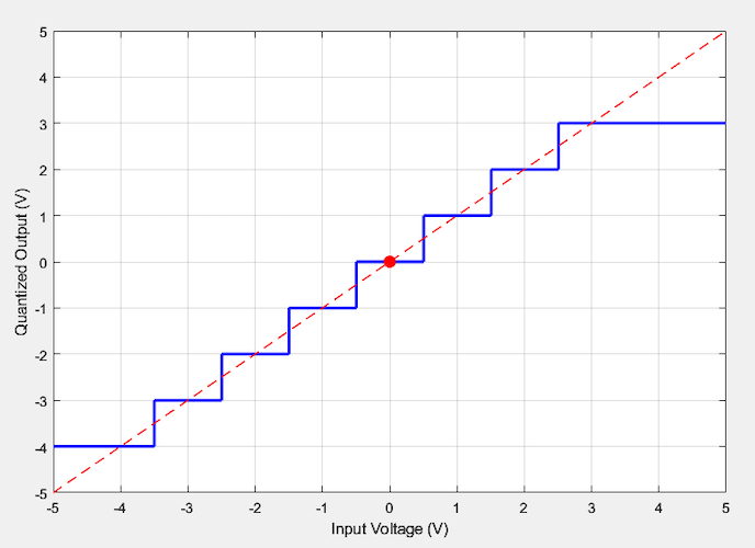
Figure 4. Illustrative uniform mid‑tread quantizer characteristic.

Any input outside the full‑scale range (±4 V) is saturated to the maximum or minimum output level. The straight line through the step midpoints approximates an ideal, infinite‑resolution quantizer and is useful for analyzing offset or gain errors of the system. For the purposes of this article, this linear model is not required.

Applying the above quantizer to the analog samples from our earlier sine‑wave example (Figure 2) produces the quantized signal shown in Figure 5.

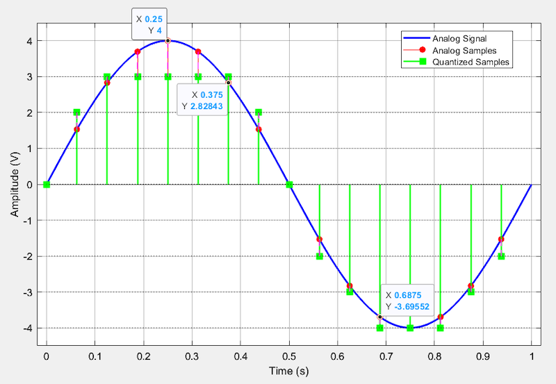
Figure 5. Original analog signal (blue) with its sampled (red) and quantized (green) values.

You can observe the quantizer’s effect through the data points. For example, because the analog samples at 0.25 s and 0.375 s exceed 2.5 V, they are both quantized to 3 V. The analog sample at 0.6875 s is less than –3.5 V, so it is quantized to –4 V, consistent with the quantizer’s input‑output characteristic. The quantizer output is therefore discrete in both time and amplitude, where each sample takes one of 8 possible discrete values.

Non-Uniform Quantization

In telephone communication systems, it’s advantageous to employ a non-uniform quantizer, where the spacing between discrete amplitude levels is not constant, as depicted in Figure 6.

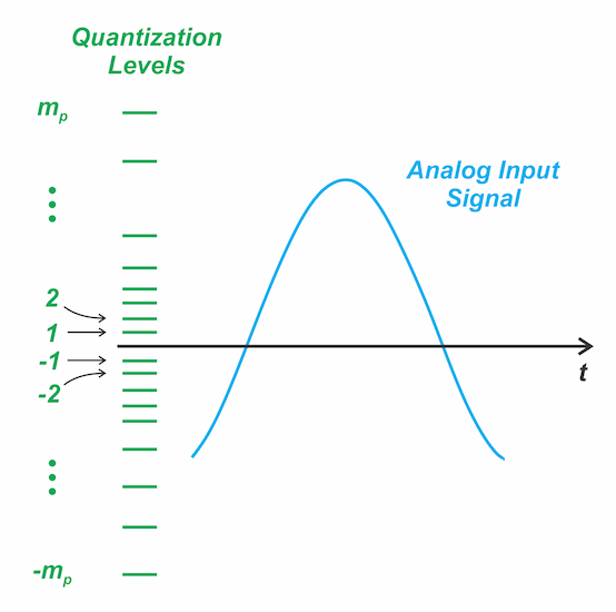
Figure 6. Non-uniform quantization.

Most speech energy lies at low amplitudes, with only occasional high‑amplitude peaks. Because these smaller amplitudes dominate statistically, non‑uniform quantization allocates more finely spaced levels in this region to better match the signal’s behavior.

In contrast, a uniform quantizer wastes many levels on rare peaks and provides too few where the signal spends most of its time, leading to poor resolution and higher distortion in soft speech segments. By allocating smaller steps for low amplitudes and larger steps for high amplitudes, non‑uniform quantization aligns the quantizer’s resolution with the actual amplitude distribution of speech.

While uniform quantization produces the same noise power at all amplitudes, the non‑uniform approach suppresses noise where the ear is most sensitive, yielding better perceived quality without increasing the bit rate. In the following articles, we will examine this non‑uniform quantization process in greater detail and explore how it is implemented in practical PCM systems.

Encoding

Sampling and quantization together transform a continuous‑time, continuous‑amplitude signal into a sequence of discrete values. To fully realize the benefits of sampling and quantization for robust signal transmission purposes, a final step is required: encoding. Encoding maps each quantized sample to a binary codeword, producing a digital bit stream.

For instance, consider a 3‑bit system in which a sample of –2 V is encoded as 010, where binary 0 is represented by 0 V and binary 1 by the supply voltage V_dd. Therefore, to transmit –2 V, the transmitter sends the sequence 0 V, V_dd, and 0 V.

At the receiver, only two voltage levels must be distinguished—not the exact analog value. Each incoming pulse is compared against a decision threshold to determine whether it represents a 0 or a 1. This simple two‑level detection strips away noise and accurately recovers the original bit stream, provided that noise remains within some limits. As a result, digital encoding is highly resilient to channel impairments, forming the foundation of modern reliable communication systems. Figure 7 shows one possible encoding for the 3-bit quantizer example.

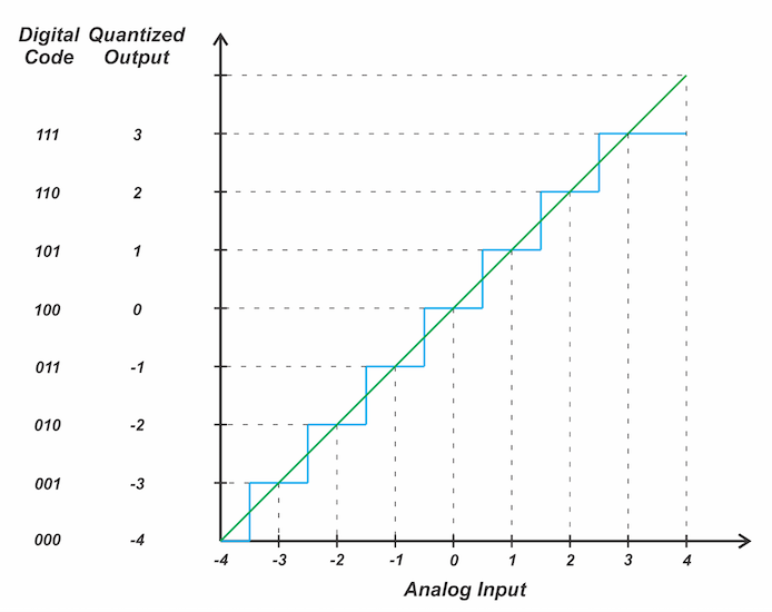
Figure 7. Encoding example for a 3‑bit quantizer.

In ADC terminology, this coding scheme is known as offset binary, where the mid‑scale code (100 in our example) corresponds to 0 V input. Codes below 100 represent negative analog voltages, while codes above 100 correspond to positive inputs.

Each PCM word is output on successive clock pulses. We call it pulse‑code modulation because, instead of transmitting the samples themselves, a pulse code or pattern is sent at each sample time to convey the information in quantized form.

Wrapping Up

In this article, we introduced pulse‑code modulation (PCM), a form of analog‑to‑digital conversion in which each instantaneous sample of an analog signal is encoded as a digital word and transmitted as a serial bit stream. PCM represents the message signal in discrete form in both time and amplitude. Three core operations produce a PCM stream: sampling, quantization, and encoding. Subsequent articles will examine each of these stages, along with the key performance trade-offs in PCM systems, in more detail.