Introduction to Non-Uniform Quantization in Pulse-Code Modulation Systems

In a previous article, we explored the basics of pulse‑code modulation (PCM), covering the key steps of sampling, quantization, and encoding. Now we turn our attention to the noise introduced by quantization, which leads us to a fundamental problem with uniform quantizers: they deliver a poor signal‑to‑noise ratio (SNR) for the low‑amplitude segments that dominate speech. Non‑uniform quantization addresses this limitation by employing variable step sizes. In this article, we'll examine how non‑uniform quantization improves SNR during soft utterances and how it is implemented in practice through compression followed by uniform quantization.

 

Quantization Error

Quantization error occurs during the analog-to-digital conversion process when continuous analog amplitudes are rounded to the nearest discrete quantization level, introducing an irreversible difference between the original and quantized signal. As an example, consider the 3‑bit quantization characteristic shown in Figure 1.

 

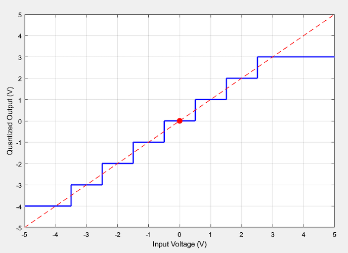
Figure 1. Illustrative uniform quantizer characteristic.

 

Figure 2 illustrates the quantization process by applying the above characteristic to the analog samples of a sine wave.

 

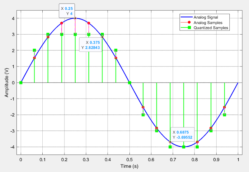
Figure 2. Analog sine wave (blue) with its sampled (red) and quantized (green) values.

 

You can observe the quantizer’s effect through the data points. For example, because the analog samples at 0.25 s and 0.375 s exceed 2.5 V, they are both quantized to 3 V. This rounding process discards fine amplitude information that cannot be recovered, making quantization error inherent to digitization, meaning that it would exist even with ideal noise‑free circuits and communication channels. The good news is that this error can be controlled. By increasing the number of quantization levels, designers can limit the quantization error to an acceptable level for the intended application.

 

Key Properties of Quantization Error

While quantization error is a deterministic signal that can be calculated exactly for a given input, it is often treated as a random additive noise source in applications like speech or music. This is illustrated in Figure 3.

 

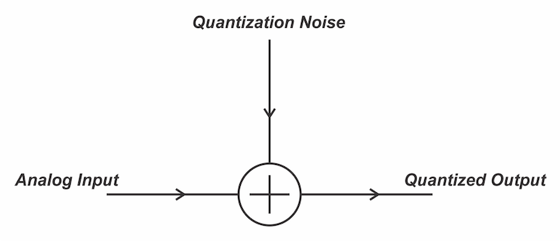
Figure 3. Quantization error modeled as a noise source.

 

This model lets us use concepts such as SNR to characterize the effect of the quantization error. However, before that, we need to understand the statistical properties of the quantization noise. A few points are worth mentioning here. 

First, the quantization error never exceeds half the step size, ±LSB/2, where LSB denotes the voltage step associated with the least significant bit. This maximum occurs when the input falls exactly midway between two quantization levels.

In addition, we can show that the noise amplitude is uniformly distributed between ±LSB/2. Since the noise amplitude is a random variable uniformly distributed between ±LSB/2, its probability density function (PDF) is shown in Figure 4.

 

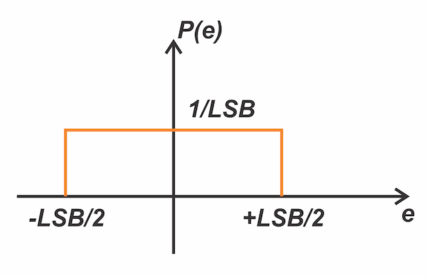
Figure 4. The probability density function of the quantization noise.

 

Note that the integral of the PDF equals one; therefore, its value is 1 / LSB for a uniform distribution over -LSB / 2 < e < LSB / 2. Given that PDF, we calculate the time-average power of the quantization noise as:

$$P_q = \int_{-LSB/2}^{+LSB/2} e^2 P(e) \ de = \int_{-LSB/2}^{+LSB/2} e^2 \times \frac{1}{LSB} \ de = \frac{LSB^2}{12}$$

Equation 1.

 

This equation gives the quantization noise power when the noise signal is uniformly distributed between ±LSB/2. As you can see, increasing the quantizer resolution reduces the LSB and the noise power.

Another important parameter of a noise source is its power spectral density, which indicates how the noise power spreads across different frequency bands. The power spectral density of the quantization noise is frequency independent. Therefore, the quantization noise is white noise with total power equal to LSB² / 12.

 

SNR Dependence on Speech Signal Power

To analyze the SNR performance of a PCM system, consider an N-bit quantizer with a full-scale range spanning from -FS to +FS. The LSB of this quantizer is:

$$LSB = \frac{2FS}{2^N} = \frac{2FS}{L}$$

Equation 2.

 

where L = 2^N denotes the total number of discrete output levels. Applying Equation 1, the quantization noise power is:

$$P_q = \frac{LSB^2}{12} = \frac{(2FS/L)^2}{12} = \frac{FS^2}{3L^2}$$

Equation 3.

 

This expression indicates that the quantization noise for a specific quantizer is a function of its full-scale value and the number of quantization levels, and is independent of the input signal power. If we denote the power of the message signal by P_s, then the SNR at the output of the quantizer is:

$$SNR = \frac{P_s}{P_q} = 3L^2 \times\frac{P_s}{FS^2}$$

Equation 4.

 

Since FS and L are fixed quantizer parameters, Equation 4 shows that the output SNR varies linearly with the message signal power. Because SNR is a direct measure of signal fidelity, this relationship means that the fidelity of the quantized signal drops as the message signal's power decreases.

In speech applications, the message signal power is subject to considerable variation. It can differ by as much as 40 dB between speakers, and is further influenced by circuit losses experienced in practical systems. Even for an individual speaker, the natural dynamics of speech feature softer utterances, which, according to Equation 4, result in a significant degradation of quantized signal quality.

 

The Predominance of Low Amplitudes in Speech Waveforms

The problem of poor SNR for weak signals becomes more important when we recognize that not all signal levels within the typical dynamic range of speech occur with the same likelihood. Statistical analysis shows that smaller amplitudes appear far more often than larger amplitudes. This is illustrated in Figure 5.

 

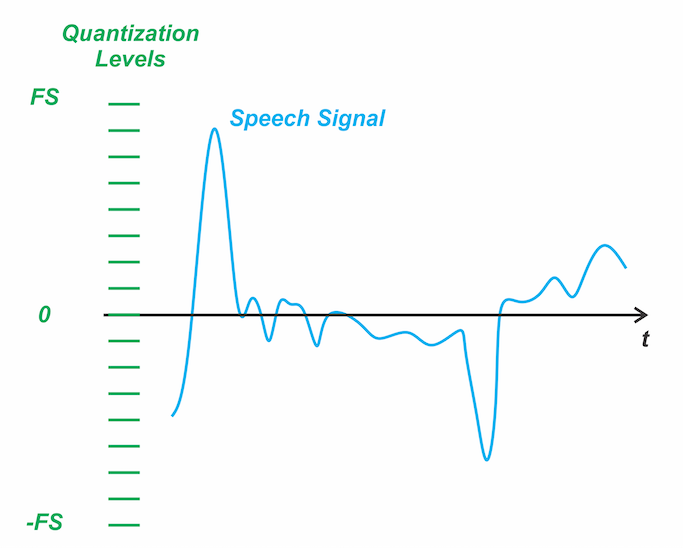
Figure 5. Using uniform quantization for speech signals.

 

Although the signal occasionally reaches high amplitudes, it spends most of its time at much lower levels. To prevent clipping, the quantizer's full-scale range must accommodate the entire dynamic range of the input signal. For a fixed number of quantization levels, this large full-scale range forces the step sizes to be relatively large. With uniform quantization, those large steps, designed to cover the full range, are applied to the low-amplitude segments where the signal spends most of its time. This leads to a coarse representation of the signal and higher quantization noise (see Equation 3).

Since quantization noise power is proportional to the square of the LSB, using a smaller LSB in the low-amplitude region improves the SNR when the signal is weak. Non‑uniform quantization applies this principle by employing smaller step sizes for low amplitudes and larger steps for high amplitudes. This allows the quantizer to allocate finer steps to the frequently occurring low‑amplitude regions while still covering the full dynamic range, as shown in Figure 6.

 

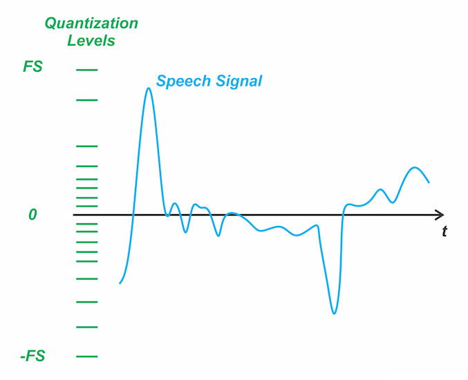
Figure 6. Variable step sizes in non‑uniform quantization.

 

While uniform quantization produces the same noise power at all amplitudes, the non‑uniform approach suppresses noise where the ear is most sensitive, yielding better perceived quality without increasing the bit rate. The SNR for large-amplitude signals will be relatively lower, but they are less frequent in speech signals. This means that during soft passages—where the signal spends most of its time—quantization noise is significantly reduced, resulting in a higher and more consistent SNR.

 

Implementing Non-Uniform Quantization Using Compression

We now examine how non-uniform quantization is realized in practice. Rather than implementing a quantizer with unequal step sizes directly, a more straightforward approach is to apply a compression characteristic to the input signal and then pass it through a uniform quantizer. This combination of compression followed by uniform quantization achieves the same effect as non-uniform quantization. To understand this, consider the example compression characteristic shown in Figure 7.

 

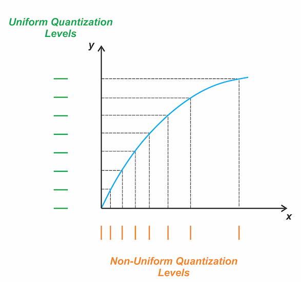
Figure 7. Compression characteristic for implementing non-uniform quantization.

 

In the curve above, the vertical steps show the equally spaced levels of the quantizer that follows the compression characteristic. By tracing these vertical steps onto the horizontal axis, we observe that one LSB of the uniform quantizer corresponds to a small input increment at low signal amplitudes, and a substantially larger increment at high amplitudes. A clear example is comparing the very first horizontal step to the very last: both correspond to one LSB of the uniform quantizer, but the actual input span for the first step is much smaller than that of the last step. The steps on the horizontal axis represent the effective non-uniform quantization levels produced by the compressor-quantizer combination. It’s evident that the step sizes increase at high amplitudes.

 

Logarithmic Compression Stabilizes SNR

With a logarithmic compression characteristic, the quantization noise becomes nearly proportional to the input signal power. As a result, the SNR remains largely independent of the input signal level. Consider the following compression characteristic to develop some intuition for why this occurs:

$$y = \ln(1 + \mu x)$$

Equation 5.

 

Here, x denotes the input voltage (for the positive portion), y is the compressed output, and μ is the compression parameter. Let Δy_i and Δx_i represent the i‑th step size on the vertical and horizontal axes, as illustrated below.

 

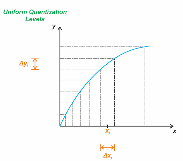
Figure 8. Determining non-uniform step sizes when using a compression characteristic.

 

To estimate the size of the i-th step, we note that the midpoint of the step, denoted by x_i, multiplied by the slope of the curve at that point, is approximately equal to a step size on the vertical axis Δy_i.

$$\Delta y_i \approx \Delta x_i \times \frac{dy}{dx}$$

Equation 6.

 

Noting that the vertical steps are all of the same size and equal to one LSB of the uniform quantizer, we have:

$$\Delta x_i \approx \frac{LSB}{dy/dx}$$

Equation 7.

 

The derivative of the logarithmic function in Equation 5 is given by:

$$\frac{dy}{dx} = \frac{ \mu}{1+ \mu x}$$

Equation 8.

 

For large μ, the derivative is proportional to 1 / x. Therefore, Equation 7 simplifies to:

$$\Delta x_i \approx LSB \times x_i$$

Equation 9.

 

Therefore, the non-uniform step size is proportional to the input signal amplitude. Since the quantization noise is proportional to the square of the step size (Δx_i)² (Equation 3), we conclude that the quantization noise is proportional to the input message power:

$$P_q \propto x_i^2 \quad \Rightarrow \quad P_q \propto P_s$$

Equation 10.

 

Because noise power scales with signal power, the SNR stays constant regardless of message power. This is exactly what we want for speech signals, where soft passages would otherwise suffer from poor SNR with uniform quantization.

Note that the above analysis is intended to provide intuition rather than serve as a rigorous mathematical proof. In practice, logarithmic compression stabilizes the SNR significantly, though it does not make it perfectly independent of the message power.

 

Wrapping Up

In this article, we examined why uniform quantization delivers poor SNR for the soft, low‑amplitude passages that dominate speech. Non‑uniform quantization addresses this by using smaller steps at low amplitudes and larger steps at high amplitudes. In practice, it is realized by passing the input signal through a compressor and then applying uniform quantization.

Logarithmic compression makes the quantization noise track the signal power, which stabilizes the SNR significantly, though it does not make it perfectly independent of message power. Two common logarithmic compression characteristics used in speech applications are μ-law (used in North America and Japan) and A-law (used in Europe and most other countries) characteristics, which will be discussed in the next article.