Understanding Pulse‑Amplitude Modulation: Natural‑Sampling Explained

In earlier installments on modulation techniques, we focused on continuous‑wave analog modulation schemes, where the message signal governs changes in a sinusoidal carrier’s amplitude, phase, or frequency. These methods, including amplitude modulation and angle modulation, provided a foundation for understanding how information can be embedded in a continuous carrier.

We now move on to a new and equally important category of modulation techniques: pulse modulation. This article opens the discussion with natural-sampling pulse‑amplitude modulation (PAM), exploring its main characteristics, such as its Fourier transform, and showing how the original message signal m(t) can be reconstructed from the modulated wave.

 

What Is Pulse‑Amplitude Modulation? A First Look

PAM is the simplest member of the analog pulse‑modulation family. It operates by sampling the message signal at regular intervals and using those sample values to set the amplitudes of a sequence of uniformly spaced pulses. Figure 1 shows the message signal together with its corresponding PAM waveform.

 

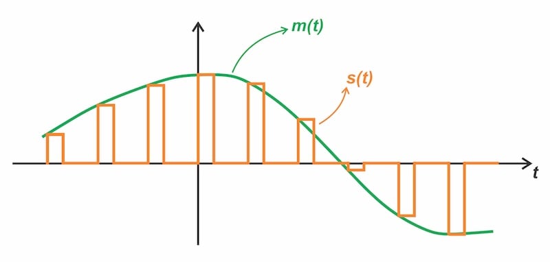
Figure 1. Message signal (green) and the corresponding PAM waveform (orange).

 

PAM shares a clear analogy with continuous‑wave amplitude modulation (AM): whereas AM varies the amplitude of a sinusoidal carrier, PAM varies the amplitudes of a sequence of pulses. Before diving into the details of PAM, it’s helpful to pause and consider why this modulation scheme is important—what, exactly, is gained by encoding information in pulse amplitudes rather than in a continuous carrier? As the next section will show, PAM serves as the basis for efficient time‑division multiplexing.

 

Why PAM Matters: Its Connection to Time‑Division Multiplexing

In communication systems, multiple‑access methods are needed to allow several users to share the same physical channel without interfering with one another. In frequency‑division multiple access (FDMA), each user is assigned a separate portion of the available spectrum, so multiple users can transmit simultaneously without interfering with one another. This is illustrated in Figure 2.

 

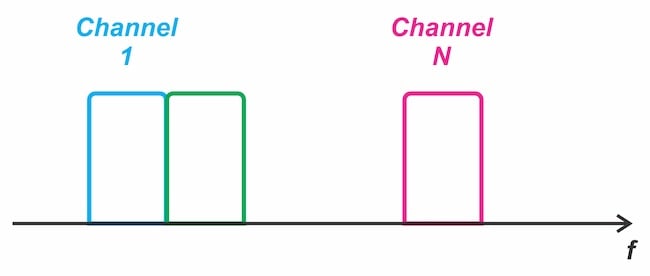
Figure 2. Frequency-division multiple access.

 

Instead of dividing the available spectrum among users, we can divide time itself and assign each user a dedicated time slot. This approach is known as time‑division multiple access (TDMA), in which all users share the same frequency band but transmit at different moments. By incorporating non‑overlapping time slots, TDMA ensures orderly access to the shared spectrum. Figure 3 depicts the fundamental idea behind TDMA.

 

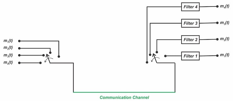
Figure 3. Application of time‑division multiplexing for transmitting multiple band‑limited signals over a single communication channel.

 

Implementing TDMA requires each user’s signal to be transmitted in short, non‑overlapping time slots, which in practice calls for pulse‑amplitude modulation (PAM) or similar pulse‑based techniques. In fact, PAM is rarely employed in single‑user communication systems because it requires a bandwidth much larger than the message bandwidth.

 

Sampling Theorem

The operation of PAM is grounded in the sampling theorem and the key insight it provides about representing continuous‑time signals through discrete samples. According to the sampling theorem, a band‑limited signal can be perfectly reconstructed from its samples as long as the sampling frequency exceeds twice the highest frequency component of the signal. This threshold, known as the Nyquist rate, guarantees that no information is lost in the sampling process and that the original waveform can be recovered exactly from the discrete sequence of samples. This insight makes it possible for PAM systems to transmit a set of samples rather than the full analog waveform.

As we’ll see, the pulse rate f_s used in PAM matches the sampling rate dictated by the sampling theorem: f_s ≥ 2B, where B denotes the highest frequency component of the analog waveform and 2B is the Nyquist rate. Having established what PAM is and why it’s important, we now turn to a deeper examination of its core concepts and properties.

 

Natural Sampling (Gating) vs. Flat-Top PAM

PAM can be generated either by natural sampling or by using flat‑top pulses. In flat‑top PAM, the pulse amplitude—set by the sampled value of the signal—remains constant throughout the pulse duration. This results in rectangular pulses with flat tops, as illustrated in Figure 1.

In natural‑sampling PAM, the pulse amplitude doesn’t remain constant over the pulse duration. Instead, it changes continuously according to the instantaneous value of the message signal. Figure 4 illustrates the natural‑sampling process by showing the original message signal m(t), the rectangular switching waveform g(t) used for gating, and the resulting natural‑sampling PAM waveform s(t).

 

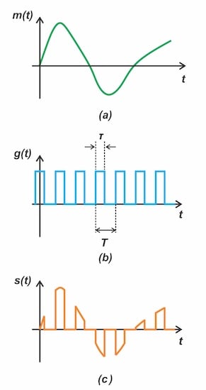
Figure 4. (a) Message signal; (b) rectangular switching waveform; (c) naturally‑sampled PAM waveform.

 

As observed, when the switching pulse is high, the output s(t) tracks the input signal, and when the pulse is low, the output is forced to zero. Therefore, natural sampling preserves the message signal’s structure, while flat‑top sampling produces a staircase‑like sequence of held sample values. Flat‑top PAM is better suited for conversion to PCM, whereas the naturally sampled form is easier to generate and finds use in other applications. As depicted in Figure 5, natural‑sampling PAM is easily implemented with an analog switch, which is a readily available component in CMOS technology.

 

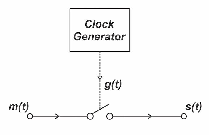
Figure 5. Using an analog switch to generate natural‑sampling PAM.

 

In the following sections, we focus on the natural‑sampling method. A subsequent article will address flat‑top PAM.

 

Spectrum of the Natural-Sampling PAM Signal

A naturally sampled PAM signal is produced by multiplying the message signal m(t) with a periodic train of rectangular pulses g(t). Hence, we have:

$$s(t) = m(t) \times g(t)$$

Equation 1.

 

The characteristics of the modulated signal can be understood by analyzing its frequency spectrum. We understand that the time‑domain multiplication corresponds to convolution of the Fourier transforms. Therefore, the Fourier transform of the modulated signal is given by:

$$S(f) = M(f) * G(f)$$

Equation 2.

 

In this expression, S(f), M(f), and G(f) represent the Fourier transforms of their respective time‑domain functions.

The next step is to determine the Fourier transform of the gating function g(t), which is a periodic rectangular pulse train of period T whose pulses have unit amplitude and remain high for τ. We place the time origin at the center of the high interval, making the waveform even and simplifying the analysis without loss of generality. Using the Fourier series representation, we can express g(t) in terms of its constituent frequency components:

$$g(t) = \sum_{n= - \infty} ^{+ \infty} c_n \ e^{jn (2 \pi / T) t}$$

Equation 3.

 

where the Fourier coefficients are given by:

$$c_n = d \ \frac{sin(n \pi d)}{n \pi d}$$

Equation 4.

 

The coefficients form a sinc‑shaped sequence that depends on the duty cycle d = τ/T. Once the Fourier series of a periodic signal is known, its Fourier transform follows directly: the transform consists of impulses at the harmonic frequencies n/T with weights equal to the Fourier‑series coefficients:

$$G(f) = \sum_{n=-\infty}^{\infty} c_n\,\delta\!\left(f - \frac{n}{T}\right)$$

Equation 5.

 

Therefore, the Fourier transform of g(t) takes the typical form illustrated in Figure 6.

 

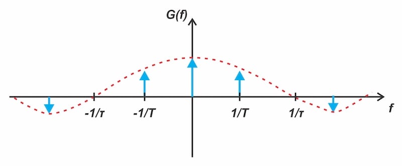
Figure 6. Typical spectrum of the rectangular switching waveform.

 

As observed, the Fourier transform of the pulse train consists of impulses at the harmonic frequencies n/T, with amplitudes following the familiar sinc envelope of a single rectangular pulse. Combining Equations 2 and 5, the Fourier transform of the modulated signal is found as:

$$S(f) = M(f) * \sum_{n=-\infty}^{\infty} c_n\,\delta\!\left(f - \frac{n}{T}\right)$$

Equation 6.

 

We need one more piece of knowledge to find the output spectrum: convolving an arbitrary spectrum M(f) with a shifted impulse δ(f − f₁) simply shifts the spectrum to the impulse’s frequency location. Hence, the output spectrum contains shifted replicas of the message spectrum at the harmonic frequencies, each scaled by the corresponding coefficient c_n. To bring the discussion together, Figure 7 uses a representative message spectrum to illustrate the typical output spectrum.

 

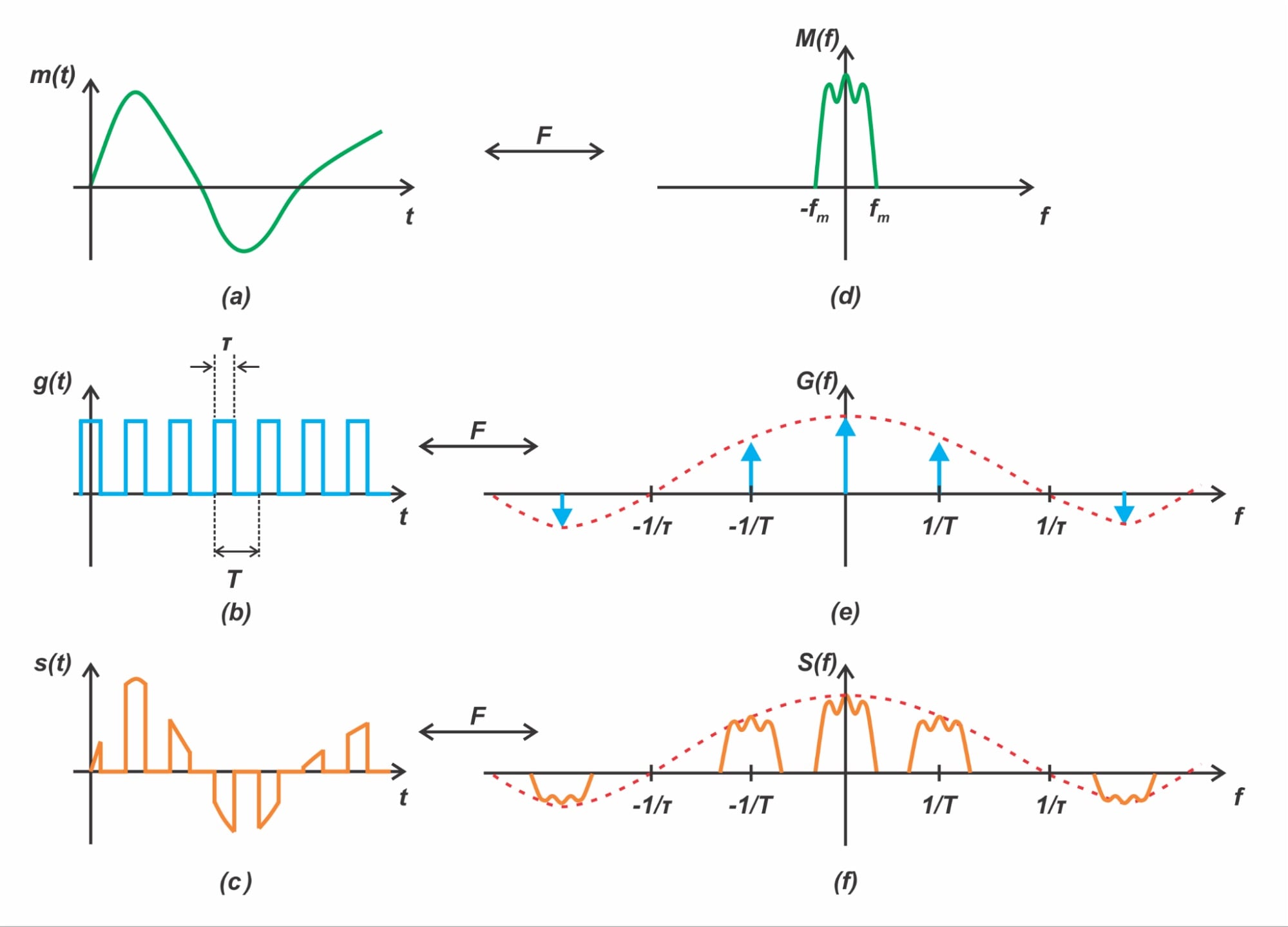
Figure 7. Illustration of natural‑sampling PAM, showing the time‑domain waveforms m(t), g(t), and s(t) together with their corresponding spectra [click to enlarge].

 

Specifically, parts (a) and (d) in the above figure show the message time-domain waveform and its spectrum; parts (b) and (e) depict the switching waveform and its spectrum; and parts (c) and (f) illustrate the modulated signal and its spectrum. A few observations are in order here:

1. From Figure 7(f), we see that to prevent overlap between the spectral replicas, the pulse rate f_s = 1/T must exceed twice the highest frequency present in the message signal, in accordance with the sampling theorem.
2. Because the spectrum of the input analog waveform is replicated at the harmonics of the sampling frequency, the resulting PAM signal occupies a bandwidth far greater than that of the original analog signal.
3. As shown in Figure 7(e), the envelope of the Fourier‑series coefficients crosses zero at 1/τ. Using the relations τ = dT and f_s = 1/T, this first null occurs at a frequency of f_s/d. Consequently, a smaller duty cycle produces a PAM signal with a wider bandwidth. Taking the null frequency f_s/d as a bandwidth indicator, we find that the spectrum extends to approximately ±3f_s when the duty cycle is d = 1/3. Moreover, if the sampling rate is chosen to be four times the message bandwidth f_m, the resulting PAM signal occupies a bandwidth roughly 12 times larger than that of the original message.

 

Recovering the Message Signal

Because the spectrum of the modulated signal consists of non‑overlapping replicas of the message spectrum, a lowpass filter with an appropriate cutoff can isolate the component around DC and recover the message signal. However, if the baseband region is corrupted by noise—for example, due to power‑supply interference or mechanical vibrations—a higher‑frequency replica may be downconverted with an analog multiplier and subsequently lowpass‑filtered to yield a cleaner reconstruction.

 

Wrapping Up

PAM transmits a sequence of constant‑width pulses whose amplitudes follow the modulating signal. These pulses are typically taken at uniformly spaced time intervals. Since PAM employs pulses, the resulting waveform has a broader bandwidth than the underlying analog signal. Despite this increase, pulse‑based schemes remain highly useful because they align naturally with digital processing and form the foundation of efficient TDM systems.