Introduction to the Gilbert Multiplier

In analog signal processing, there is often a requirement for a circuit that accepts two analog inputs and generates an output proportional to their product. These analog multiplier circuits find applications in communication systems, squarers, frequency doublers, and high-frequency power measurement. They also play a crucial role in implementing phase detectors in phase-locked loops (PLLs) that work with sine-wave inputs and sine-wave voltage-controlled oscillators.

Most integrated circuit multipliers are based on a structure known as the Gilbert cell. In this article, we'll examine the basic concept and operation of the Gilbert multiplier. To provide the necessary background, however, let's start with a simpler multiplier.

 

Emitter-Coupled Pair as a Simple Multiplier

Analog multiplication can be performed using a differential amplifier with a variable transconductance. The Gilbert cell is a modified version of this circuit, which is illustrated in Figure 1.

 

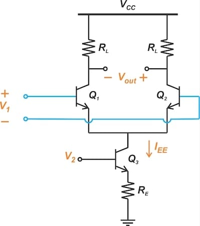
Figure 1. An emitter-coupled pair functions as a simple analog multiplier. Image used courtesy of Steve Arar

 

In this circuit, one input (V₁) is applied to the differential pair. The other input (V₂) is used to control the current through the differential pair.

A differential pair is a nonlinear circuit. However, for a small V₁, the circuit behaves as a constant-gain amplifier. Under the assumption that V₁ is small and the bias current (I_EE) is fixed, the output voltage can be expressed as:

$$V_{out} ~\approx~ g_m R_L V_1$$

Equation 1.

 

where g_m denotes the transconductance of each transistor in the differential pair, as given by:

$$g_m ~=~ \frac{I_c}{V_T} ~=~ \frac{I_{EE}}{2V_T}$$

Equation 2.

 

In the above equation, I_c denotes the collector current, and V_T is the thermal voltage. The bias current of the emitter-coupled pair is given by:

$$I_{EE} ~=~ \frac{V_2 - V_{BE}}{R_E} ~\approx~ \frac{V_2}{R_E}$$

Equation 3.

 

where V_BE is the voltage drop across the base-emitter junction. Note that the approximation in Equation 3 assumes that V₂ is much greater than V_BE (about 0.7 V).

Combining Equations 1 through 3, the output voltage may be expressed as:

$$V_{out} ~\approx~ \frac{R_L}{2 R_E V_T} ~\times~ V_1 V_2$$

Equation 4.

 

which shows that the output voltage is proportional to the product of the two input signals.

Before we move on to discussing the Gilbert multiplier, a few points are worth bringing up here. For one thing, it's important to remember that Equation 4 relies on Equations 1 through 3. It is therefore only valid if V₁ is small (Equation 1) and V₂ ≫ V_BE (Equation 3).

Because V₂ must remain positive, the multiplier function is limited to only two quadrants of the V₁-V₂ plane. For that reason, the basic emitter-coupled pair is often referred to as a two-quadrant multiplier. One- and two-quadrant multipliers typically have simpler circuitry compared to four-quadrant multipliers.

 

Finally, although it may not be immediately obvious, a fundamental characteristic that enables an emitter-coupled pair to act as a multiplier is that the transconductance of a bipolar transistor is proportional to its collector current (see Equation 2). This relationship between the collector current (I_c) and the transconductance (g_m) results from the exponential transfer function of bipolar transistors.

Given that g_m is proportional to I_c, we create a multiplier by making I_c proportional to the second input voltage (V₂). As a result, the emitter-coupled pair requires bipolar transistors. This is also true of the original Gilbert multiplier, which is the circuit we'll examine in the rest of this article.

 

The Gilbert Multiplier: Simplified Analysis

The Gilbert multiplier is a modified emitter-coupled pair that can perform four-quadrant multiplication. Its core structure is shown in Figure 2.

 

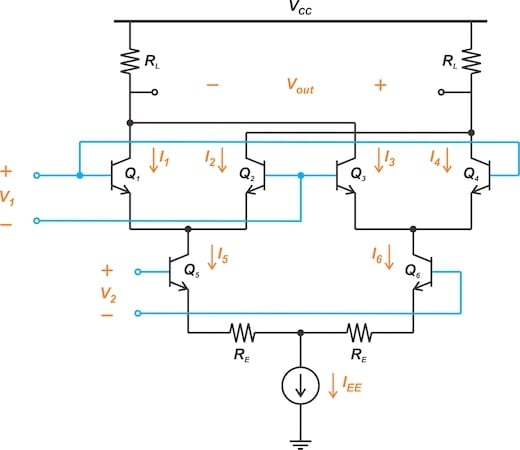
Figure 2. The core configuration of a Gilbert multiplier. Image used courtesy of Steve Arar

 

To accurately analyze the above circuit, we must take into account the exponential transfer function of the bipolar transistors. However, using a linear model for the transistors still yields useful insights into the circuit's operation.

Let's take a look at the simplified analysis. With the currents shown in Figure 2, the output voltage is:

$$\begin{eqnarray} V_o &~=~& -R_L (I_2 ~+~ I_4) ~+~ R_L (I_1 ~+~ I_3) \\ &~=~& R_L \Big ( (I_1 ~-~ I_2) ~+~ (I_3 ~-~ I_4) \Big ) \end{eqnarray}$$

Equation 5.

 

Assuming that V₁ is a small signal, we have:

$$I_1 ~-~ I_2 ~=~ g_{m1}V_1 \quad \text{and} \quad I_4 ~-~ I_3 ~=~ g_{m3}V_1$$

Equation 6.

 

where:

g_m1 is the transconductance of the transistors Q₁ and Q₂

g_m3 is the transconductance of the transistors Q₃ and Q₄.

Substituting Equation 6 into Equation 5, we obtain:

$$V_o ~=~ R_L \Big ( g_{m1}V_1 ~-~ g_{m3}V_1 \Big ) ~=~ R_L V_1 (g_{m1}~-~g_{m3})$$

Equation 7.

 

Assuming that the bias currents through Q₁ and Q₂ are I₅/2 and the bias currents through Q₃ and Q₄ are I₆/2, we may express the transconductances g_m1 and g_m3 as:

$$g_{m1} ~=~ \frac{I_5}{2V_T} \quad \text{and} \quad g_{m3} ~=~ \frac{I_6}{2V_T}$$

Equation 8.

 

Combining Equations 7 and 8 produces:

$$V_o ~=~ \frac{R_L V_1}{2V_T} (I_5 ~-~ I_6)$$

Equation 9.

 

Applying Kirchhoff's Voltage Law in the loop that includes V₂ and the base-emitter junctions of Q₅ and Q₆, we have:

$$V_2 ~=~ V_{BE,5} ~+~ R_E I_5 ~-~ R_E I_6 ~-~ V_{BE,6} ~\approx~ R_E (I_5 ~-~ I_6)$$

Equation 10.

 

Combining the last two equations, we have:

$$V_o ~=~ \frac{R_L}{2R_E V_T} ~\times~ V_1 V_2$$

Equation 11.

 

which indicates that the circuit operates as a multiplier.

 

A More Exact Analysis

In the previous section, we examined a Gilbert multiplier with emitter degeneration resistors (R_E). In this section, we'll analyze a Gilbert cell configuration that lacks these resistors (Figure 3).

In addition, we will no longer assume that the input voltages are small. Therefore, we can no longer use linear models for the bipolar transistors. Though this requires that we use the exponential transfer functions, for the sake of simplicity we'll skip the mathematical derivations.

 

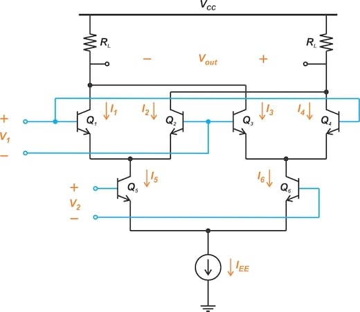
Figure 3. The Gilbert cell without emitter degeneration resistors. Image used courtesy of Steve Arar

 

The output voltage of this configuration is proportional to the product of the hyperbolic tangents of the two inputs:

$$V_{out} ~=~ R_L I_{T} \Big [ \tanh \big ( \frac{V_1}{2 V_T} \big) \ \tanh \big ( \frac{V_2}{2 V_T} \big) \Big ]$$

Equation 12.

 

The hyperbolic tangent function can be approximated by its argument when the argument is small. Therefore, assuming that V₁ and V₂ are both much less than 2V_T, the above equation can be approximated as:

$$V_{out} ~\approx~ R_L I_{T} \big ( \frac{V_1}{2 V_T} \big) \big ( \frac{V_2}{2 V_T} \big)$$

Equation 13.

 

which indicates that the circuit operates as a multiplier.

The pertinent question is this: How can we perform accurate multiplication when the inputs are larger than 2V_T?

As we know from fundamental analog design courses, emitter degeneration resistors can help linearize the input-output characteristics of a transistor. We saw previously that emitter degeneration resistors can be added to the differential pair consisting of Q₅ and Q₆. Therefore, if only one of the inputs is greater than 2V_T, we can use the circuit shown in Figure 2 and apply the larger input to the lower differential pair.

However, it should be noted that emitter degeneration can't be used with the cross-coupled differential pairs (transistors Q₁ through Q₄). To understand this, recall that the Gilbert cell depends on the exponential transfer function of bipolar transistors. This makes each transistor's transconductance proportional to its collector current.

To perform accurate multiplication when V₁ is not much smaller than 2V_T, it's possible to pass V₁ through a predistortion circuit so that the nonlinearity of the predistorter compensates for that of the multiplier circuit.

From Equation 12, the nonlinearity of the multiplier is in the form of a hyperbolic tangent. Therefore, the predistortion circuit should exhibit an inverse hyperbolic tangent characteristic. Although creating this type of predistortion circuit may seem daunting at first, its implementation using bipolar transistors is quite straightforward.

We'll skip these details because of space constraints, but those interested can refer to the book "Analysis and Design of Analog Integrated Circuits" by Paul R. Gray et al.

 

Implementing Arithmetic Functions With Op Amps and Multipliers

Multipliers, including the Gilbert multiplier, can be utilized within the feedback loop of an op amp to develop a range of useful functions. The fundamental concept is that by applying the output of an op amp to a specific function, F(x), and feeding the result back to the inverting input of the op amp, the amplifier's output will yield the inverse function F⁻¹(x). For instance, by placing a Gilbert cell in the feedback path, we can implement an analog divider. This is illustrated in Figure 4.

 

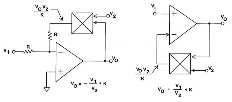
Figure 4. Implementing analog dividers by utilizing Gilbert cells in the feedback path of op amps. Image used courtesy of Analog Devices

 

Note that the configuration on the left produces an inverting divider, whereas the configuration on the right is a non-inverting divider.

 

Wrapping Up

The exponential transfer function of bipolar transistors results in a transconductance that is proportional to the collector current. This fundamental property is what enables the Gilbert cell to act as a multiplier. Without employing linearization methods, accurate multiplication with the Gilbert cell requires both inputs to be well below 2V_T. Multipliers can be employed in the feedback loop of operational amplifiers to create a variety of useful circuits, including analog dividers.