 Facebook
 Google
 GitHub
 Linkedin
Max & Math: Maxwell’s Equations in Relativistic Times
Maxwell's equations, which summarize the interaction of electromagnetic fields, have always been described using the "math of the times." Using tensors, they can be given in two equations!
Here's the story of how Maxwell's theories on the interaction of electromagnetic fields went from being expressed in 12 equations to two.
Maxwell's equations become more compact as math becomes more modern. Maxwell originally presented 20 equations using partial differentials. Using vectors, Heaviside needed four equations to express the same ideas. Now, using tensors and 4D "relativistic" notation, only two equations are needed. Let's take a look.
If you're not familiar with Maxwell's equations, you might want to start here: Maxwell’s Equations in Present Form.
Classical Foundations
In 1864, James Clerk Maxwell presented to the world a new entity: the electromagnetic field. He was the first to mathematically describe the interaction of electric and magnetic fields. He went on to identify light as a form of electromagnetic energy. The partial differential equations he used were the "state of the art" for his time, circa the 1860s.
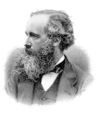
A portrait of James Clerk Maxwell by G. J. Stodart.
Maxwell was aware that the math was a stumbling block to his theories being readily accepted. He attempted their first reformulation using quaternions developed by William Hamilton. Quaternions could be used to describe 3D rotations and, while Maxwell felt they described his theories better, they did not make the math easier.
Quaternions fell out of favor with mathematicians towards the end of the 19th century, but they've found modern use in 3D computer game development. Processing quaternions allows for better smoothing functions.
It wasn't until 1884 when Oliver Heaviside reformulated the 12 equations describing electromagnetic phenomena that Maxwell's work began to be understood. Using his vector analysis, Heaviside turned Maxwell's original 12 equations into four.
These are the familiar four equations that are usually referred to as Maxwell's equations. With Maxwell's theories expressed in vectors, the scientific community began to appreciate the value of Maxwell's contributions. Researchers around the world focused on creating electromagnetic waves.
In 1888, Heinrich Hertz was able to produce electromagnetic waves outside of the visible spectrum, thereby proving Maxwell's theories.
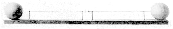
The dipole resonator Hertz created trying to prove Maxwell's theories. From Electrical Communication Magazine, 1927.
Looking at the vector equations, you might think that was the wrap up for Maxwell's equations: four neatly packaged equations that describe the interaction of electric and magnetic fields and their relationship to optics.
But what about photons? Particles? Charges moving near the speed of light? What do the equations say about these phenomena? Not much—science continues to progress, but the equations have stayed the same.
Heaviside's Formulations: The Starting Point
The vector versions of Maxwell's equations were just a starting point. The insights Maxwell gave to the world were finally in a form where the math was understandable. From Hertz taking on the task of proving Maxwell's theories until today, the equations have motivated scientists and engineers.
Check any of the top technical universities and you'll find active research concerning electromagnetic phenomena. Currently, research focus is on interactions of the Electromagnetic + Weak + Strong forces and the Higgs boson.
Vector reformulations, relativity, quantum physics, and quantum field theory have emerged. Mathematical structures, as well as entire branches of study, also emerged to describe and analyze the complex interactions of moving charges, magnetic fields, and electromagnetic energy.
One area of active research in the early 19th century was how to deal with complex 3D objects. When Einstein was working on his theory of general relativity, the complexity of curved space-time had him seeking methods for describing and transforming objects. Vectors were useful in local frames of reference; Einstein was working with observers in different frames of reference. Different observers were "looking" at the same object from different frames of reference—one electrical, one magnetic, one system at rest, one moving.
When Einstein became aware of tensors, he saw possibilities.
Tensor Calculus
Gregorio Ricci-Curbustro developed a branch of mathematics rooted in absolute differential calculus. He is the one responsible for establishing the foundations of tensor calculus.
In the early 1900s, his student Tullio Levi-Civita published the book The Absolute Differential Calculus (Calculus of Tensors). Tensors did not depend on a field of reference; they presented a structure that could be described and manipulated between frames of reference. Einstein learned tensor calculus and even developed a system of indexes that allowed objects to be described mathematically. Einstein used tensors throughout his paper on general relativity, published in 1915.
What tensors do is allow more complex operations to be described and handled similarly to simpler calculations. Once in tensor form, the object can be manipulated in accordance with the rules of tensor calculus. Tensors also allow for transformations and manipulations regardless of the frame of reference. The components that make up tensors may change with the frame of reference, but, taken as a whole, a tensor in one frame of reference is the same physical object in another frame of reference.
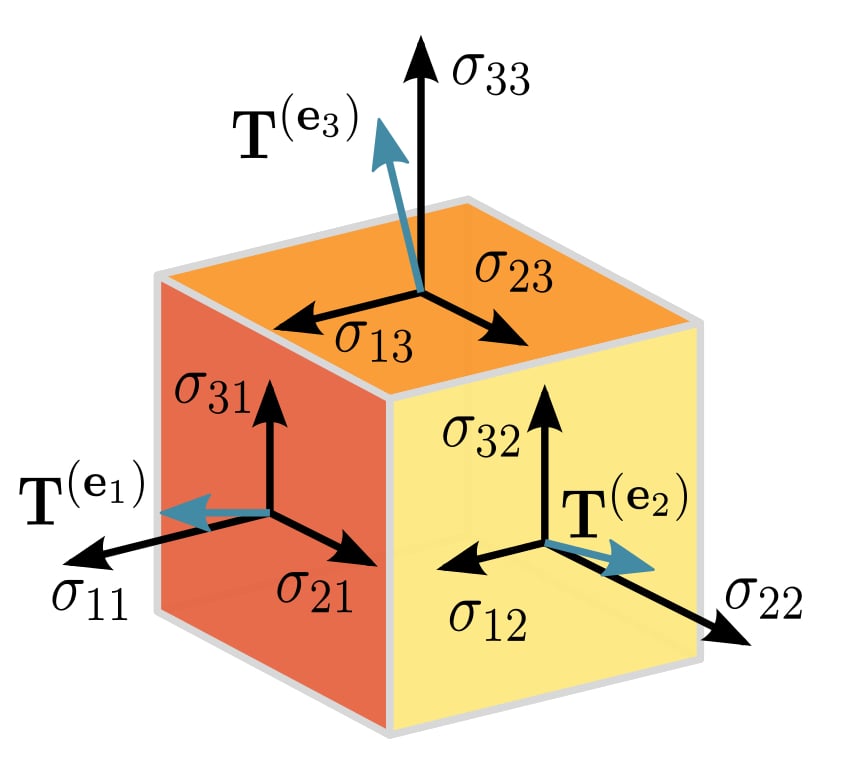
An example of a visualized second-order tensor. Image courtesy of Timothy Rias, derived from original work by Sanpaz [CC BY-SA 3.0]
As mathematical systems advance in complexity, as their structures incorporate more information, they allow for more compact ways of expressing ideas. Vectors condensed Maxwell's 12 original equations into four. Tensors allow them to be expressed in two!
We've seen examples from the information technology field in which more complex data structures allow data to be handled easily. Instead of referring to a specific person by first, middle, and last name with titles and other associated information, we can create a data structure labeled "NameField." This data structure can contain the information that allows us to design systems using and manipulating the NameField without getting mired in the actual details of the components of the name.
Incorporating that NameField into an advanced data structure with even more information labeled "Person" allows for even easier conceptualization of people. The more complex structures incorporate even more information and provide better organization.
The same ideas apply when using advanced mathematical structures. The structures carry the information components within them.
Tensors are represented mathematically as arrays. The number of indices of the array is referred to as the rank or order of the tensor. To label an individual component of the array, you need that many indices. A tensor of rank 4 is represented by a 4×4 array. For each component, you need to provide the indices for its position in the array. The first component may be labeled A1,1,1,1.
Tensors of rank 0 are scalars (numbers); rank 1 are vectors (a column of numbers); rank 2 are matrices (columns and rows); and finally, there are multi-dimensional arrays of rank n.
Rank: Name:
0 Scalar
1 Vector
2 Matrix
n n-Tensor
The mathematical operations that tensors follow change depending on the rank of the tensor. There are operations specific for vectors, matrices, 3-tensors, 4-tensors, and n-tensors.
Working with Four Dimensions
In a relativistic system, the basic coordinates have four dimensions (t, x, y, z), with time as the additional component. Cartesian three-dimensional systems have just three components (x, y, z).
The electric and magnetic fields which are considered separate entities in a classical system become components of a single antisymmetric 4×4 tensor in a relativistic system. In the classical view, the electric field was a vector and the magnetic field a pseudo-vector.
Note: The following images of equations are courtesy of Wikipedia.
The electromagnetic tensor is described as follows:
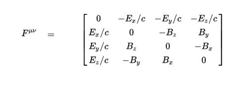
Notice there are only components of the electric and magnetic fields as unknowns; notice also that the speed of light is involved.
Using this tensor, one equation can describe Gauss's Law and the Ampere-Maxwell Law (for β = 1, 2, 3):
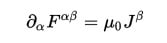
where
$$J^{\beta}$$ = ( cp Jx Jy Jz), the charge and current density four-vector.
This field tensor equation covers two vector equations:
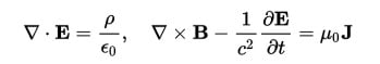
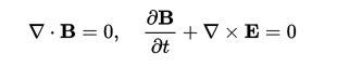
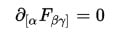
The other two vector equations express Gauss's Law for Magnetism and Faraday's Law:
These can be reduced to the Bianchi identity:
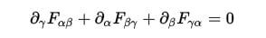
which, using relativistic notation, can be given as
More Maxwell
So, is that it for Maxwell's original equations? NO!
These tensor formulations are only one way to present Maxwell's equations. And in addition to the influence of different mathematical approaches, physicists look at electromagnetic phenomena one way, mathematicians another.
You'll see equations for vacuums (where, without matter, charge and current densities are zero). There will be equations for specific boundary conditions, initial conditions, surface conditions, with and without specific timeframes. Within small-scale quantum systems, wave-particle reformulations are used; when working with photons in quantum field theory, electric and magnetic fields do not appear in the equations.
Why are the classical equations still taught? The classical equations are still valid when dealing with non-relativistic velocities at normal scales—i.e., the context in which most of our engineering problems exist. The vector equations give correct answers for many engineering problems, and the math is simpler than with the advanced equations.
At the heart of all the math are the physical phenomena of electromagnetic energy—how moving charges give rise to a self-sustaining wave propagating at the speed of light. This was Maxwell's true gift.
Summary
Tensor calculus allows Maxwell's equations to be reformulated using the electromagnetic tensor in two equations. There are many ways to present Maxwell's equations, and mathematical structures are still being developed for analyzing electromagnetic phenomena. The classical equations, however, are still valid for most engineering problems, and this is why they are still used.
Related Content


Good article. I always thought his middle name was Clerk, not Clark.