 Facebook
 Google
 GitHub
 Linkedin
Simulating Non-linear Transformers in LTspice
Learn how to use non-linear models in LTspice to simulate the characteristics of transformers, a crucial part of SMPS (switched-mode power supply) design.
In a previous article, we learned how to model inductors with LTspice. We saw three options to model inductors, each with different complexity and accuracy. When designing circuits that contain inductors we need to take into account real phenomena such as hysteresis or inductor saturation. In order to get it, we can make use of the Chan model, which has already shown great accuracy.
While LTspice comes with models to simulate Chan inductors and other non-linear models, it is not possible to simulate arbitrary coupled inductors (transformers). However, there are some techniques to do it.
This article shows how to implement non-linear models and how to extend them to any circuit. Simulating the real characteristics of transformers is critical in the design of switched-mode power supplies (SMPSs). Practical examples are provided, as well as the files to replicate all the simulations.
Transformers
An ideal transformer consists of at least two windings that are mutually coupled. To set a transformer in LTpsice, place two inductances L1, L2 and then, define the Mutual Coupling (K) through a Spice directive.
The phase dots will automatically show up once you define the directive. An ideal transformer has mutual coupling equal to one, while real ones present lower values, as it is later explained.
![]()
Figure 1. The ideal transformer in LTspice
Non-linear Transformers
Once we know how to model ideal transformers, we can start including complex parameters in the simulation model, so we go towards a real behavior.
Hysteresis
Magnetic materials tend to stay magnetized after having experienced a field force, even after this has been removed. The relationship between the flux density (B) and the field intensity (H) is shown in the hysteresis loop. The most relevant points of a hysteresis loop are saturation (in both directions), retentivity, coercivity. The size and shape of the hysteresis loops are directly dependent upon the type of magnetic material.
![]()
Figure 2. Hysteresis loop of an inductor. Images used courtesy of the NDT Resource Center and LTWiki
The two hysteresis loop branches can be modeled with two equations. One for the upper branch and for the lower one:
\[B_+ (H) = B_s \frac{H+H_c}{{\vert{H+H_{c}} \vert + H_c}(\frac{B_s}{B_r} - 1)} , B_- (H) = B_s \frac{H-H_c}{{\vert{H-H_{c}} \vert + H_c}(\frac{B_s}{B_r} - 1)}\]
The Chan model shows that it is possible to model hysteresis using three magnetic parameters.
- Coercive force (amps-turns/m), Hc.
- Remnant flux density (T), Br.
- Saturation flux density (T), Bs.
Besides, we need to consider the physical aspects of the transformer:
- Magnetic Length (Lm), in meters
- Length of the gap (Lg), in meters
- Cross-sectional area (A), in square meters
- Number of turns (N)
The main drawback of using this model for simulations is the difficulty to get the value of these parameters. Some manufacturers of magnetic cores directly provide them, otherwise, you would need to infer them. It is also possible to measure the B-H curves using an oscilloscope or other specific instrumentation.
Parasitic Components
Real transformers have parasitic elements that limit their use in real life. Parasitics determine aspects such as the physical shape or windings orientation. Besides, parasitic elements will limit the frequency operation of transformers. We can model parasitic elements with the following circuit:
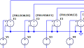
![]()
Figure 3. Parasitic elements of a transformer
- Leakage inductance L3, L4. The imperfect coupling between the primary L1 and the secondary L2 is translated into a self-inductance in series in both primary and secondary windings.
Leakage inductances can be explicit with the coupling coefficient K, which determines how well are both inductances coupled:
\[K = \sqrt{ \frac{L1L2}{(L1+L3)(L2+L4)}}\]
- Winding capacitances C1, C2. These come from the coupling between the windings and the magnetic core as well as from the winding of consecutive turns.
- Coupling capacitances C3, C4. In this case, they appear because of the physical proximity between the primary and the secondary winding(s).
- Wire resistance R1, R2. Wirings, usually made by copper, have a non-infinite resistivity, provoking ohmic losses.
When designing a transformer, it is usual that the modification of one of the parasitic elements has an impact on another one. Hence, when simulating the effect of parasitic elements, it is very interesting to study their impact on the whole circuit making them variable. It can be done by setting them as parameters and using the directive STEP.
Simulating Non-linear Transformers
Even LTspice does not allow to simulate arbitrary coupled inductors, there are some workarounds to get non-linear transformers simulated. The easiest way is to model a perfect transformer using controlled sources and then, add in parallel the non-ideal inductor. The following circuit can be packed in a subcircuit (subckt) and used in any other simulation where a transformer is needed.
![]()
Figure 4. Non-linear transformer circuit in LTspice
Simulating Ideal vs Non-ideal Transformers
A simple circuit containing an ideal transformer can be as follows:
![]()
Figure 5. Simulating a circuit with an ideal transformer in LTspice
The coupling between the primary and the secondary windings is perfect, and both windings are purely inductive. They have the same inductance value, so the current induced in the secondary winding should have the same value that circulates through the primary winding. Comparing the voltage induced in the secondary winding with the primary one, we can see that there is no distortion and that the amplitude is exactly the same.
![]()
Figure 6. Primary and secondary waveforms in a circuit with an ideal transformer
Furthermore, we can check that this behavior keeps the same even if we continue increasing the input current because the ideal inductor never arrives at saturation.
Repeating the process with a non-linear transformer, we see that the waveforms get distorted when we keep increasing the current. The behaviors are very different, so taking some time to simulate non-ideal conditions really worth the effort.
![]()
Figure 7. Simulating a circuit with a non-ideal transformer
![]()
Figure 8. Primary and secondary waveforms in a circuit with a non-ideal transformer
Tips and Tricks
- In the non-ideal transformer circuit, the Chan model can be replaced by any other model for inductors. Since obtaining the Chan parameters can be sometimes difficult, for some applications, the flux model can be good enough.
- When simulating a non-ideal transformer with the Chan model, we do not know its inductance. You can measure it by placing a current source with a known slope at the transformer input and then measuring the voltage \[(V = -L \frac{dI}{dt})\].
- LTspice comes with a variety of examples which are a good start point for any analysis. You can find them in the folder: examples\educational in the LTspice installation’s folder.
Files
Click to download:


I don’t understand this article. A transformer is in most cases voltage-driven, and using 2Hz is not at all representative of a practical case.
One can see easily that the default DCR of the linear inductors totally overwhelms the reactance.
If I use the circuit in fig3, how should I assign the parameter of “K”? Is It “K L1 L2 1”?