Facebook
 Google
 GitHub
 Linkedin
Understanding Amplitude Quantization Error for ADCs
This article examines the quantization error of an analog-to-digital converter.
This article examines the quantization error of an analog-to-digital converter.
An ADC transforms an input value into one of the values from a set of discrete levels and outputs a digital code to specify the quantization level. The quantization process introduces some error into the system.
This article will look at quantization error by applying a ramp input to a quantizer. Then, we’ll look at an example in which the quantization error resembles a noise source. Moreover, we’ll discuss the advantages of modeling the quantization error using a noise source. We’ll continue this discussion in the next part of this article. There, we’ll look at the assumptions that allow us to use the noise model, and we’ll use the obtained model to characterize the effect of the quantization error.
An Ideal ADC
The transfer function of an ideal unipolar three-bit ADC is shown in Figure 1.
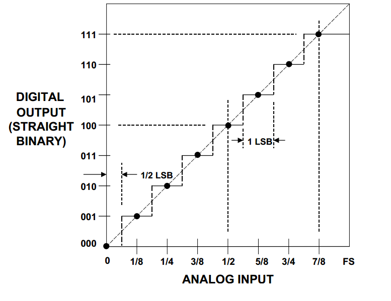
Figure 1 Image courtesy of Analog Devices.
The full scale (FS) value of the analog input is divided into eight equal intervals (denoted by ⅛, ¼, ...). At the mid-point of these intervals, there is a transition from one digital output value to the next one. Except for the first and the last steps, the other steps have a width equal to FS/8. The width of the steps (FS/8) also specifies the analog value of the least significant bit (LSB) of the output digital code. Hence, if we apply the output of the above ADC to an ideal digital-to-analog converter (Figure 2), the code 001 will produce the analog value FS/8, the code 010 will produce FS/4, and so on.
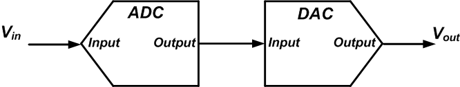
Figure 2
Amplitude Quantization Error
The important point here is that a given digital code represents a range of analog input values; the amplitude of the input is quantized. For example, all the input values ranging from FS/16 to 3*FS/16 are represented by one output code (the code 001). If we connect the output of the ADC to an ideal three-bit DAC (Figure 2), the code 001 will produce the analog value FS/8. Hence, the analog values ranging from FS/16 to 3*FS/16 are represented by a single analog value FS/8. Therefore, even ideal amplitude quantization introduces some error. This error is called quantization error (Vq) and can be calculated by subtracting the ADC input (Vin) from the output of the DAC (Vout) as shown in Figure 3 below.
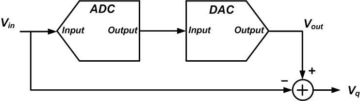
Figure 3
Quantization Error for a Ramp Input
Let’s apply a ramp signal to the input of the above setup and examine the quantization error more closely. The blue line in Figure 4 shows the ramp applied to the input. Moreover, the figure shows the quantized levels that we get in the DAC output in red.
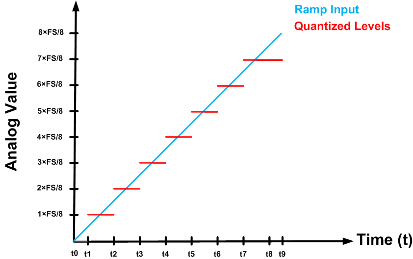
Figure 4
Between t0 and t1, the input is less than FS/16. Considering the input-output characteristic of Figure 1, the ADC output is 000 which gives the quantized analog value Vout=0. As shown in Figure 5, the quantization error goes from 0 to - ½ ✕ FS/8 (minus half LSB) for this interval.
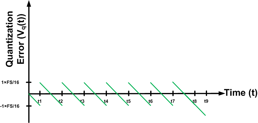
Figure 5
Between t1 and t2, the input is greater than FS/16 and less than 3FS/16. The ADC output is 001 which gives the quantized analog value Vout=FS/8 (See Figure 1 and 4). For this interval, the quantization error ranges from + ½ ✕ FS/8 to - ½ ✕ FS/8 (See Figure 5). Similarly, we can find the error value for the other quantization levels as shown in Figure 5. Note that except for the last level, the quantization error is always between ± FS/16 (half LSB).
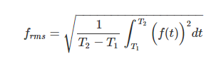
Now we can use Figure 5 to calculate the root mean square (RMS) value of the quantization error for a ramp input. The RMS of a function f(t) defined over the interval T1 < t < T2 is obtained by the following equation:
For the error waveform of Figure 5, we have:
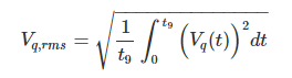
To keep things simple, we ignore the first part (0 < t < t1) and the last part (t8 < t < t9) of the waveform. The error introduced by ignoring these two parts decreases as the resolution of the quantizer increases. We obtain:
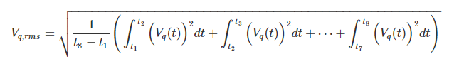
The integrals in the above equation correspond to the time-shifted versions of the same signal. A time shift doesn’t change the area under a curve (or equivalently, its integral). Therefore, these integral terms are equal. Since t2-t1 = t3-t2 = …= t8-t7, we can simplify the above equation as:
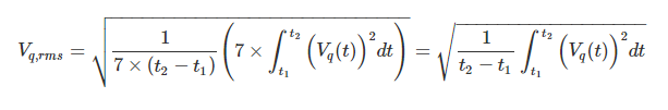
Equation 1
We can directly calculate the above integral. However, to make the calculations simpler, we assume that t2-t1 = T and apply a time shift of -T/2 to the waveform. Hence, we can simply calculate the RMS of Vq,new(t) shown in Figure 6 below.

Figure 6
Therefore, Equation 1 can be rewritten as
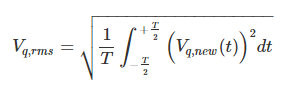
Equation 2
where Vq,new(t) is given by the following equation:
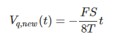
Substituting this equation into Equation 2 and doing the math gives
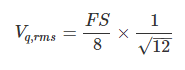
We know that FS/8 is the analog value of the LSB. Therefore, the RMS error is given by the following equation:
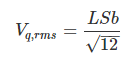
This is an important result and we’ll derive it one more time later (in the second part of this article) looking at the problem from a different point of view.
Let’s summarize our findings so far: We saw that even ideal amplitude quantization introduces some error, called quantization error, into the system. To investigate some properties of this error, we applied a ramp input and observed that the RMS of the error is proportional to the LSB value. Also, as depicted in the example of Figure 5, the quantization error is always between ±LSB/2. Increasing the resolution of the quantizer will reduce the LSB and the error term. Moreover, ignoring the first part (0 < t < t1) and the last part (t8 < t < t9) of the waveform in Figure 5, we observe that the mean value of the error is zero. Also note that, for a given value of the input, we can calculate the exact value of the error.
Quantization Error for a More Complicated Input
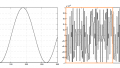
Although the above discussion allows us to gain insight into some properties of the quantization error, it’s based on an unrealistic assumption, namely, that the input is a ramp. Let’s have a look at another example. This time we quantize the discrete cosine signal x[n]=0.99cos(n/10) depicted in Figure 7.
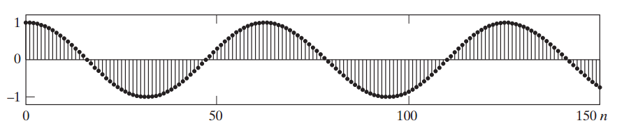
Figure 7 Image courtesy of Discrete-Time Signal Processing.
If we apply an eight-bit quantizer to this signal, the quantization error sequence will be as shown in Figure 8.
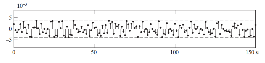
Figure 8 Image courtesy of Discrete-Time Signal Processing.
Unlike the case of the ramp input, the error for this example doesn’t seem to follow a pattern and it’s not easy to calculate the RMS error. Comparing the input cosine of this example with the error sequence, we observe the following:
- The input is a single-frequency signal, but the frequency content of the error signal seems quite different. It has rapid variations, so we expect it to have high-frequency components.
- We cannot recognize a connection between the input cosine and the error sequence by visual inspection. It seems that the error sequence is not correlated with the input and varies randomly from one sample to the next.
As we observed in the example of the ramp input, we know that the quantization error signal is not really random and can, in fact, be calculated for a given input value. But what if we could model the quantization error as a random signal under some assumptions? The amplitude of the quantization error is between ±LSB/2, which can be a small value, particularly when we’re dealing with a high-resolution quantizer. Now, if this low-amplitude signal varies in an unpredictable manner, one may conclude that it resembles the noise sources that we usually encounter in different circuits and systems.
Advantages of Modeling Quantization Error as a Noise Source
Considering the quantization error as a noise source can simplify the problem a lot. We know how to analyze the effect of particular types of noise sources on a linear time-invariant (LTI) system. The instantaneous value of a noise source is usually unpredictable, so a time-domain analysis is not possible. However, we can observe the noise for a long time and use measured results to find a statistical model of the noise. For example, a helpful characteristic of a noise source is its “power spectral density” (PSD), which allows us to gain insight into the average power of the noise in different frequency bands. Having the PSD of a noise signal, we can use the Laplace transform (for a continuous-time system) or the Z transform (for a discrete-time system) to analyze the effect of the noise on the output spectrum of an LTI system (without knowing the instantaneous value of the noise).
Hence, assuming that it’s possible to model the quantization process by a noise source, we only need to find the power spectral density of the noise model and use it to characterize the effect of the error on the performance of the system. In this case, we can use the model of Figure 3 to describe the quantization process with an additive noise source, as shown in Figure 9. As you can see, the quantized value (Vout) is equal to the input (Vin) plus a noise signal that models the quantization error (Vq).
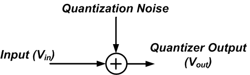
Figure 9
In the next part of this article, we’ll examine the conditions under which we can model the quantization error as a noise source. Then, we’ll dive into some important characteristics of the obtained model and use them to analyze the effect of quantization error on system performance.
Conclusion
Even ideal amplitude quantization introduces some error, called quantization error, into the system. The RMS of this error is proportional to the LSB value. It seems that we can model the quantization error as a noise signal under certain assumptions. If possible, this can significantly simplify analyzing the effect of quantization error on system performance.
To see a complete list of my articles, please visit this page.