Quantization Noise and Amplitude Quantization Error in ADCs

Learn the methods and applications of modeling the quantization error of an ADC using a noise source.

In the previous article on quantization error for ADC converters, we observed that, for particular cases, the quantization error resembles a noise signal. We also discussed that modeling the error term as a noise signal can significantly simplify the problem of analyzing the effect of the error on system performance.

In this article, we’ll look at the conditions under which we are allowed to use a noise source to model the quantization error. Then, we’ll discuss the statistical model of the quantization noise and use it to analyze the quantization error.

When Does a Noise Model Lead to Valid Results?

We can easily find examples where the quantization error is predictable and doesn’t act as a noise source. For example, if the input of a quantizer is a DC value, the quantization error will be constant. As another example, assume that the amplitude of the input is always between two adjacent quantization levels of the quantizer. In this case, the quantization error is equal to the input minus a DC value.

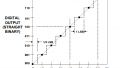
Another interesting case occurs when the input is a sinusoid and the sampling frequency of the quantizer is a multiple of the input frequency. An example is illustrated in Figure 1 below.

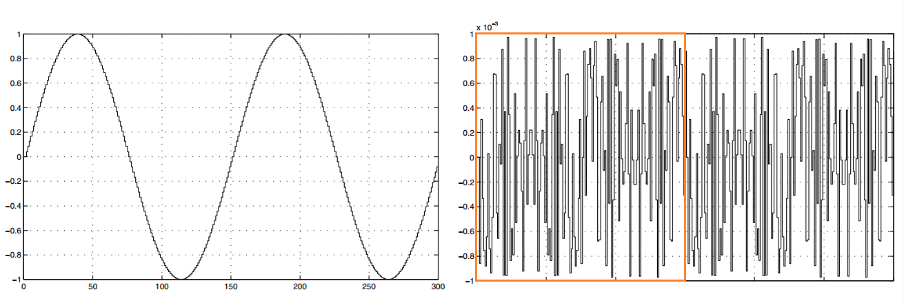
Figure 1. Image courtesy of Data Converters.

The left curve of Figure 1 depicts two periods of a 10-bit quantized sine wave. The right curve shows the quantization error. For this example, the ratio of the sampling frequency to the input frequency is 150.

Visual inspection of the quantization error reveals periodic behavior (one period is indicated by the orange rectangle). As you can see, there is a correlation between the input and the error signal, whereas a noise source is not correlated with the input. In such cases, we expect the error signal to have considerable frequency components at the harmonics of the input.

The error signal does not resemble noise in the above examples. However, in many practical applications, such as speech or music, the input is a complicated signal and exhibits rapid fluctuations that occur in a somewhat unpredictable manner. In such cases, the error signal is likely to act as a noise source.

Experimental measurements and theoretical studies have shown that modeling the quantization error as a noise source is valid if the following four conditions are satisfied:

1. The input approaches the different quantization level values with equal probability (in some of the problematic examples discussed above, we saw that the input was always near some particular quantization levels).
2. The quantization error is not correlated with the input.
3. The quantizer has a large number of quantization levels (such as when we have a high-resolution ADC).
4. The quantization steps are uniform (unlike the data converters used in telephony that have a logarithmic characteristic).

You can find a more formal way of expressing these conditions in Section 4.8.3 of the book Discrete-Time Signal Processing.

If these necessary conditions are satisfied, we can replace the error signal with an additive noise source as shown in Figure 2. This allows us to use concepts such as signal-to-noise ratio (SNR) to characterize the effect of the quantization error. However, before that, we need to find a statistical model for the noise source.

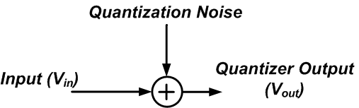
Figure 2

Statistical Model of Quantization Noise

The first step in characterizing a noise source can be estimating how often a given value is likely to occur. This amplitude distribution can be obtained by observing the noise signal for a long time and taking samples to create an amplitude histogram. The histogram consists of a number of bins that correspond to the contiguous amplitude intervals spanning the entire possible range of the noise amplitude. The height of a bin indicates the number of samples that lie in the bin interval.

Let’s take a look at an example histogram of quantization noise. Assume that the input is the discrete cosine signal x[n]=0.99cos(n/10) (shown in Figure 3).

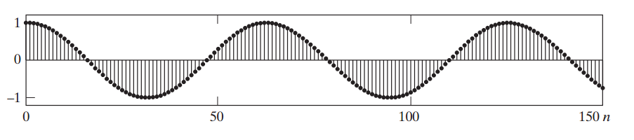
Figure 3. Image courtesy of Discrete-Time Signal Processing.    

If we apply an eight-bit quantizer to this signal, the quantization error sequence will be as shown in Figure 4.

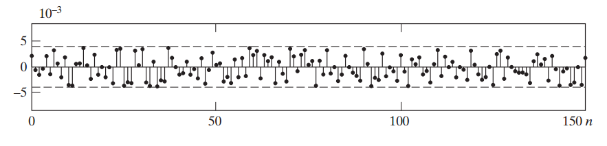
Figure 4. Image courtesy of Discrete-Time Signal Processing.

The Quantization Noise Amplitude Distribution

Now, we take 101,000 samples from the error signal and construct a histogram with 101 bins that represent amplitude intervals ranging from -LSB/2 to +LSB/2.

The result is shown in Figure 5 below.

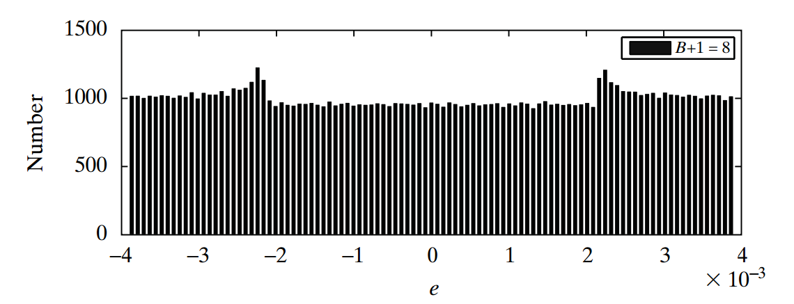
Figure 5. Image courtesy of Discrete-Time Signal Processing.

As you can see, LSB/2 is about 4×10^-3 for this example.

Interestingly, almost the same number of samples lie in the different bin intervals; the height of the bins is close to the total number of samples (101,000) divided by the number of bins (101). In other words, the noise amplitude is uniformly distributed between ±LSB/2. If we increase the quantizer resolution, we’ll get an even more uniform amplitude distribution. This is consistent with the third prerequisite for a valid noise model.

While we examined the histogram for a particular case of input type and quantizer resolution, the result is valid for other cases in which the quantization error acts as a noise source. Hence, we can assume that the noise amplitude is a random variable uniformly distributed between ±LSB/2.

The probability density function will be as shown in Figure 6.

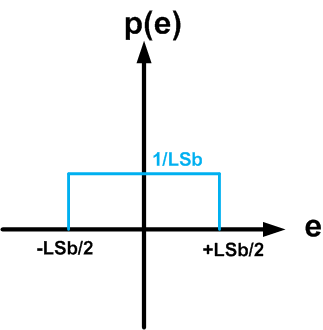
Figure 6

The quantization noise can take a value between ±LSB/2, and the probability density function is constant in this range (i.e., it’s a uniform distribution). Since the integral of the probability density function is equal to one, its value will be 1/LSB for -LSB/2 < e < LSB/2 (see Figure 6).

Now, we can calculate the time average power of the quantization noise as

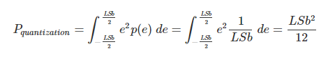
Equation 1

This equation gives us the quantization noise power when the noise signal is uniformly distributed between ±LSB/2. As you can see, increasing the resolution of the quantizer will reduce the LSB and the noise power. Note that this equation is consistent with the RMS value that we obtained (in the previous article) for the quantization error of a ramp input.

Quantization Noise Power Spectral Density

The other important parameter of a noise source is the power spectral density, which indicates how the noise power spreads in different frequency bands. To find the power spectral density, we need to calculate the Fourier transform of the autocorrelation function of the noise.

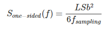
Assuming that the noise samples are not correlated with one another, we can approximate the autocorrelation function with a delta function in the time domain. Since the Fourier transform of a delta function is equal to one, the power spectral density will be frequency independent. Therefore, the quantization noise is white noise with total power equal to LSB²/12.

To find the one-sided power spectral density, S_one-sided(f), over the Nyquist interval (DC to f_sampling/2), we should divide the noise power by f_sampling/2. Hence,

How Does Quantization Degrade SNR?

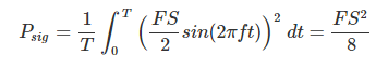
Now that we know the power and power spectral density of the quantization noise, we can use the model of Figure 2 to analyze the quantization process. For example, assume that we have an N-bit quantizer with full-scale value denoted by FS. What will the SNR at the quantizer output be if we apply the sinusoid $$\frac{FS}{2}sin(2\pi ft)$$ to the quantizer? The output will be the input sinusoid plus some noise produced by the quantization process. The desired signal power can be calculated as

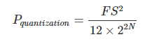
The power of the quantization noise is given by Equation 1. We only need to replace LSB with $$\frac{FS}{2^N}$$. Therefore, the noise power is

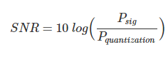
The SNR is given by the following equation:

Plugging in the values, we obtain

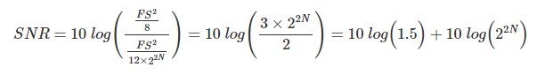
This leads to the following expression:

Equation 2

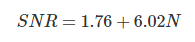
This is an important equation that allows us to determine the maximum SNR of an ideal N-bit quantizer when the input is a sine wave with the maximum possible amplitude (FS/2). For example, based on Equation 2, we know that the maximum SNR of a 10-bit ADC is about 60 dB. Note that each additional bit of resolution increases the SNR by 6.02 dB.

Equation 2 takes only the quantization noise into account. If there is any other noise source in the system, the SNR will be lower than what Equation 2 predicts. For example, although we expect a 10-bit ADC to have an SNR of about 60 dB, the noise from electronic components can lead to a lower SNR. Assume that such additional noise sources reduce the SNR of our 10-bit ADC to 55.94 dB.

In this case, we can plug the ADC SNR into Equation 2 to determine the effective resolution of the ADC, which is usually referred to as the “effective number of bits” (ENOB).

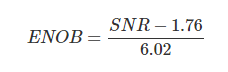
Hence, if a 10-bit ADC exhibits an SNR of 55.94 dB, its ENOB is 9 bits.

As a final note, remember that Equation 2 is derived by assuming that the band of interest is the Nyquist interval. If the input signal has a bandwidth lower than the Nyquist frequency, we may be able to select only the band of interest from the quantizer output and improve the effective SNR of the data converter.

Summary

• Under certain assumptions, we are allowed to model the quantization error as a noise source.
• The quantization noise amplitude is a random variable uniformly distributed between ±LSB/2.
• With a uniform amplitude distribution, the quantization noise power is equal to $$\frac{LSB^2}{12}$$.
• The power spectral density of the quantization noise is frequency independent (it’s white noise).
• For a sine wave, we can find the maximum SNR of an ideal N-bit quantizer as SNR=1.76+6.02N.

To see a complete list of my articles, please visit this page.