 Facebook
 Google
 GitHub
 Linkedin
Square Wave Signals
It has been found that any repeating, non-sinusoidal waveform can be equated to a combination of DC voltage, sine waves, and/or cosine waves (sine waves with a 90 degree phase shift) at various amplitudes and frequencies.
This is true no matter how strange or convoluted the waveform in question may be. So long as it repeats itself regularly over time, it is reducible to this series of sinusoidal waves.
In particular, it has been found that square waves are mathematically equivalent to the sum of a sine wave at that same frequency, plus an infinite series of odd-multiple frequency sine waves at diminishing amplitude:
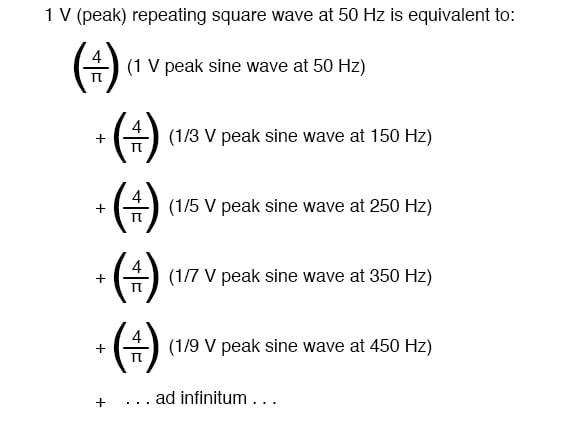
This truth about waveforms at first may seem too strange to believe. However, if a square wave is actually an infinite series of sine wave harmonics added together, it stands to reason that we should be able to prove this by adding together several sine wave harmonics to produce a close approximation of a square wave.
This reasoning is not only sound, but easily demonstrated with SPICE.
The circuit we’ll be simulating is nothing more than several sine wave AC voltage sources of the proper amplitudes and frequencies connected together in series. We’ll use SPICE to plot the voltage waveforms across successive additions of voltage sources, like this:
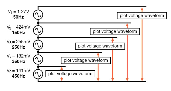
A square wave is approximated by the sum of harmonics.
In this particular SPICE simulation, I’ve summed the 1st, 3rd, 5th, 7th, and 9th harmonic voltage sources in series for a total of five AC voltage sources. The fundamental frequency is 50 Hz and each harmonic is, of course, an integer multiple of that frequency.
The amplitude (voltage) figures are not random numbers; rather, they have been arrived at through the equations shown in the frequency series (the fraction 4/π multiplied by 1, 1/3, 1/5, 1/7, etc. for each of the increasing odd harmonics).
building a squarewave
v1 1 0 sin (0 1.27324 50 0 0)       1st harmonic (50 Hz)
v3 2 1 sin (0 424.413m 150 0 0)     3rd harmonic
v5 3 2 sin (0 254.648m 250 0 0)     5th harmonic
v7 4 3 sin (0 181.891m 350 0 0)     7th harmonic
v9 5 4 sin (0 141.471m 450 0 0)     9th harmonic
r1 5 0 10k
.tran 1m 20m
.plot tran v(1,0)    Plot 1st harmonic
.plot tran v(2,0)    Plot 1st + 3rd harmonics
.plot tran v(3,0)    Plot 1st + 3rd + 5th harmonics
.plot tran v(4,0)    Plot 1st + 3rd + 5th + 7th harmonics
.plot tran v(5,0)    Plot 1st + . . . + 9th harmonics
.end
I’ll narrate the analysis step by step from here, explaining what it is we’re looking at. In this first plot, we see the fundamental-frequency sine-wave of 50 Hz by itself. It is nothing but a pure sine shape, with no additional harmonic content. This is the kind of waveform produced by an ideal AC power source:
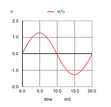
Pure 50 Hz sinewave.
Next, we see what happens when this clean and simple waveform is combined with the third harmonic (three times 50 Hz, or 150 Hz). Suddenly, it doesn’t look like a clean sine wave any more:
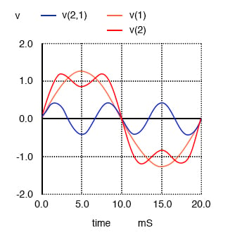
Sum of 1st (50 Hz) and 3rd (150 Hz) harmonics approximates a 50 Hz square wave.
The rise and fall times between positive and negative cycles are much steeper now, and the crests of the wave are closer to becoming flat like a squarewave. Watch what happens as we add the next odd harmonic frequency:
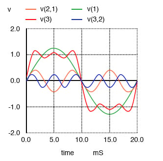
Sum of 1st, 3rd and 5th harmonics approximates square wave.
The most noticeable change here is how the crests of the wave have flattened even more. There are more several dips and crests at each end of the wave, but those dips and crests are smaller in amplitude than they were before. Watch again as we add the next odd harmonic waveform to the mix:
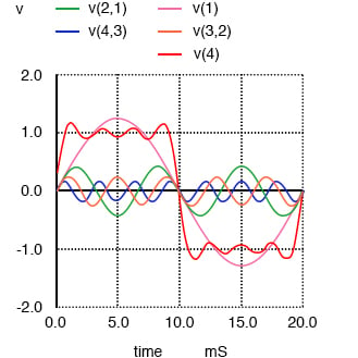
Sum of 1st, 3rd, 5th, and 7th harmonics approximates square wave.
Here we can see the wave becoming flatter at each peak. Finally, adding the 9th harmonic, the fifth sine wave voltage source in our circuit, we obtain this result:
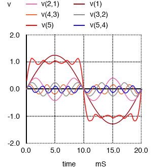
Sum of 1st, 3rd, 5th, 7th and 9th harmonics approximates square wave.
The end result of adding the first five odd harmonic waveforms together (all at the proper amplitudes, of course) is a close approximation of a square wave. The point in doing this is to illustrate how we can build a square wave up from multiple sine waves at different frequencies, to prove that a pure square wave is actually equivalent to a series of sine waves.
When a square wave AC voltage is applied to a circuit with reactive components (capacitors and inductors), those components react as if they were being exposed to several sine wave voltages of different frequencies, which in fact they are.
The fact that repeating, non-sinusoidal waves are equivalent to a definite series of additive DC voltage, sine waves, and/or cosine waves is a consequence of how waves work: a fundamental property of all wave-related phenomena, electrical or otherwise.
The mathematical process of reducing a non-sinusoidal wave into these constituent frequencies is called Fourier analysis, the details of which are well beyond the scope of this text. However, computer algorithms have been created to perform this analysis at high speeds on real waveforms, and its application in AC power quality and signal analysis is widespread.
SPICE has the ability to sample a waveform and reduce it into its constituent sine wave harmonics by way of a Fourier Transform algorithm, outputting the frequency analysis as a table of numbers. Let’s try this on a square wave, which we already know is composed of odd-harmonic sine waves:
squarewave analysis netlist
 v1 1 0 pulse (-1 1 0 .1m .1m 10m 20m)
 r1 1 0 10k
 .tran 1m 40m
 .plot tran v(1,0)
 .four 50 v(1,0)
 .end
The pulse option in the netlist line describing voltage source v1 instructs SPICE to simulate a square-shaped “pulse” waveform, in this case one that is symmetrical (equal time for each half-cycle) and has a peak amplitude of 1 volt. First we’ll plot the square wave to be analyzed:
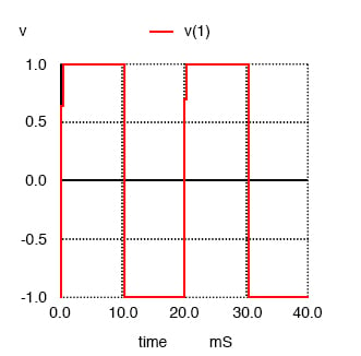
Squarewave for SPICE Fourier analysis
Next, we’ll print the Fourier analysis generated by SPICE for this square wave:
fourier components of transient response v(1)
dc component =  -2.439E-02
harmonic  frequency   fourier     normalized   phase   normalized
no          (hz)     component    component    (deg)   phase (deg)
1         5.000E+01   1.274E+00     1.000000    -2.195       0.000
2         1.000E+02   4.892E-02     0.038415   -94.390     -92.195
3         1.500E+02   4.253E-01     0.333987    -6.585      -4.390
4         2.000E+02   4.936E-02     0.038757   -98.780     -96.585
5         2.500E+02   2.562E-01     0.201179   -10.976      -8.780
6         3.000E+02   5.010E-02     0.039337  -103.171    -100.976
7         3.500E+02   1.841E-01     0.144549   -15.366     -13.171
8         4.000E+02   5.116E-02     0.040175  -107.561    -105.366
9         4.500E+02   1.443E-01     0.113316   -19.756     -17.561
total harmonic distortion =     43.805747  percent
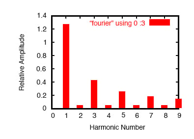
Plot of Fourier analysis results.
Here, (Figure above) SPICE has broken the waveform down into a spectrum of sinusoidal frequencies up to the ninth harmonic, plus a small DC voltage labelled DC component.
I had to inform SPICE of the fundamental frequency (for a square wave with a 20 millisecond period, this frequency is 50 Hz), so it knew how to classify the harmonics. Note how small the figures are for all the even harmonics (2nd, 4th, 6th, 8th), and how the amplitudes of the odd harmonics diminish (1st is largest, 9th is smallest).
This same technique of “Fourier Transformation” is often used in computerized power instrumentation, sampling the AC waveform(s) and determining the harmonic content thereof. A common computer algorithm (sequence of program steps to perform a task) for this is the Fast Fourier Transform or FFT function.
You need not be concerned with exactly how these computer routines work, but be aware of their existence and application.
This same mathematical technique used in SPICE to analyze the harmonic content of waves can be applied to the technical analysis of music: breaking up any particular sound into its constituent sine-wave frequencies.
In fact, you may have already seen a device designed to do just that without realizing what it was! A graphic equalizer is a piece of high-fidelity stereo equipment that controls (and sometimes displays) the nature of music’s harmonic content.
Equipped with several knobs or slide levers, the equalizer is able to selectively attenuate (reduce) the amplitude of certain frequencies present in music, to “customize” the sound for the listener’s benefit. Typically, there will be a “bar graph” display next to each control lever, displaying the amplitude of each particular frequency.
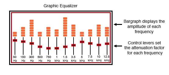
Hi-Fi audio graphic equalizer.
A device built strictly to display—not control—the amplitudes of each frequency range for a mixed-frequency signal is typically called a spectrum analyzer.
The design of spectrum analyzers may be as simple as a set of “filter” circuits (see the next chapter for details) designed to separate the different frequencies from each other, or as complex as a special-purpose digital computer running an FFT algorithm to mathematically split the signal into its harmonic components.
Spectrum analyzers are often designed to analyze extremely high-frequency signals, such as those produced by radio transmitters and computer network hardware. In that form, they often have an appearance like that of an oscilloscope:
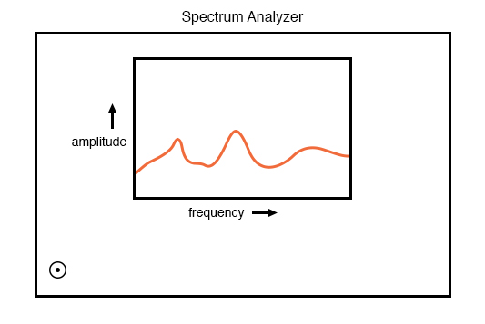
Spectrum analyzer shows amplitude as a function of frequency.
Like an oscilloscope, the spectrum analyzer uses a CRT (or a computer display mimicking a CRT) to display a plot of the signal.
Unlike an oscilloscope, this plot is amplitude over frequency rather than amplitude over time. In essence, a frequency analyzer gives the operator a Bode plot of the signal: something an engineer might call a frequency-domain rather than a time-domain analysis.
The term “domain” is mathematical: a sophisticated word to describe the horizontal axis of a graph. Thus, an oscilloscope’s plot of amplitude (vertical) over time (horizontal) is a “time-domain” analysis, whereas a spectrum analyzer’s plot of amplitude (vertical) over frequency (horizontal) is a “frequency-domain” analysis.
When we use SPICE to plot signal amplitude (either voltage or current amplitude) over a range of frequencies, we are performing frequency-domain analysis.
Please take note of how the Fourier analysis from the last SPICE simulation isn’t “perfect.” Ideally, the amplitudes of all the even harmonics should be absolutely zero, and so should the DC component. Again, this is not so much a quirk of SPICE as it is a property of waveforms in general.
A waveform of infinite duration (infinite number of cycles) can be analyzed with absolute precision, but the less cycles available to the computer for analysis, the less precise the analysis. It is only when we have an equation describing a waveform in its entirety that Fourier analysis can reduce it to a definite series of sinusoidal waveforms.
The fewer times that a wave cycles, the less certain its frequency is. Taking this concept to its logical extreme, a short pulse—a waveform that doesn’t even complete a cycle—actually has no frequency, but rather acts as an infinite range of frequencies. This principle is common to all wave-based phenomena, not just AC voltages and currents.
Suffice it to say that the number of cycles and the certainty of a waveform’s frequency component(s) are directly related.
We could improve the precision of our analysis here by letting the wave oscillate on and on for many cycles, and the result would be a spectrum analysis more consistent with the ideal. In the following analysis, I’ve omitted the waveform plot for brevity’s sake—its just a really long square wave:
square wave
v1 1 0 pulse (-1 1 0 .1m .1m 10m 20m)
r1 1 0 10k
.option limpts=1001
.tran 1m 1
.plot tran v(1,0)
.four 50 v(1,0)
.end
fourier components of transient response v(1)
dc component =   9.999E-03
harmonic  frequency    fourier    normalized   phase   normalized
no           (hz)     component   component    (deg)   phase (deg)
1         5.000E+01   1.273E+00     1.000000    -1.800       0.000
2         1.000E+02   1.999E-02     0.015704    86.382      88.182
3         1.500E+02   4.238E-01     0.332897    -5.400      -3.600
4         2.000E+02   1.997E-02     0.015688    82.764      84.564
5         2.500E+02   2.536E-01     0.199215    -9.000      -7.200
6         3.000E+02   1.994E-02     0.015663    79.146      80.946
7         3.500E+02   1.804E-01     0.141737   -12.600     -10.800
8         4.000E+02   1.989E-02     0.015627    75.529      77.329
9         4.500E+02   1.396E-01     0.109662   -16.199     -14.399
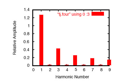
Improved fourier analysis.
Notice how this analysis (Figure above) shows less of a DC component voltage and lower amplitudes for each of the even harmonic frequency sine waves, all because we let the computer sample more cycles of the wave. Again, the imprecision of the first analysis is not so much a flaw in SPICE as it is a fundamental property of waves and of signal analysis.
REVIEW:
- Square waves are equivalent to a sine wave at the same (fundamental) frequency added to an infinite series of odd-multiple sine-wave harmonics at decreasing amplitudes.
- Computer algorithms exist which are able to sample waveshapes and determine their constituent sinusoidal components. The Fourier Transform algorithm (particularly the Fast Fourier Transform, or FFT) is commonly used in computer circuit simulation programs such as SPICE and in electronic metering equipment for determining power quality.
RELATED WORKSHEETS:


So, when did time get measured in millisiemens (mS), or in this case 50 Ohms? I guess I found this a little confusing.
In the first calculation, what does 4π represent?