Facebook
 Google
 GitHub
 Linkedin
Other Waveshapes
As strange as it may seem, any repeating, non-sinusoidal waveform is actually equivalent to a series of sinusoidal waveforms of different amplitudes and frequencies added together. Square waves are a very common and well-understood case, but not the only one.
Electronic power control devices such as transistors and silicon-controlled rectifiers (SCRs) often produce voltage and current waveforms that are essentially chopped-up versions of the otherwise “clean” (pure) sine-wave AC from the power supply.
These devices have the ability to suddenly change their resistance with the application of a control signal voltage or current, thus “turning on” or “turning off” almost instantaneously, producing current waveforms bearing little resemblance to the source voltage waveform powering the circuit.
These current waveforms then produce changes in the voltage waveform to other circuit components, due to voltage drops created by the non-sinusoidal current through circuit impedances.
Nonlinear Components
Circuit components that distort the normal sine-wave shape of AC voltage or current are called nonlinear. Nonlinear components such as SCRs find popular use in power electronics due to their ability to regulate large amounts of electrical power without dissipating much heat.
While this is an advantage from the perspective of energy efficiency, the waveshape distortions they introduce can cause problems.
These non-sinusoidal waveforms, regardless of their actual shape, are equivalent to a series of sinusoidal waveforms of higher (harmonic) frequencies.
If not taken into consideration by the circuit designer, these harmonic waveforms created by electronic switching components may cause erratic circuit behavior.
It is becoming increasingly common in the electric power industry to observe overheating of transformers and motors due to distortions in the sine-wave shape of the AC power line voltage stemming from “switching” loads such as computers and high-efficiency lights.
This is no theoretical exercise: it is very real and potentially very troublesome.
In this section, I will investigate a few of the more common waveshapes and show their harmonic components by way of Fourier analysis using SPICE.
One very common way harmonics are generated in an AC power system is when AC is converted, or “rectified” into DC. This is generally done with components called diodes, which only allow the passage of current in one direction.
Half-wave Rectification
The simplest type of AC/DC rectification is half-wave, where a single diode blocks half of the AC current (over time) from passing through the load. (Figure below)
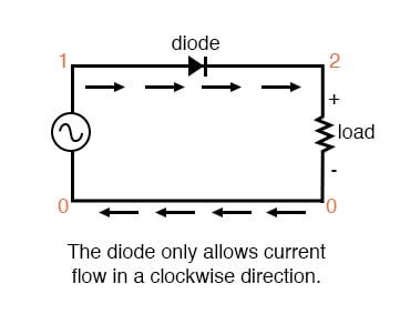
Half-wave rectifier
halfwave rectifier
v1 1 0 sin(0 15 60 0 0)
rload 2 0 10k
d1 1 2 mod1
.model mod1 d
.tran .5m 17m
.plot tran v(1,0) v(2,0)
.four 60 v(1,0) v(2,0)
.end
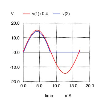
Half-wave rectifier waveforms. V(1)+0.4 shifts the sine wave input V(1) up for clarity. This is not part of the simulation.
First, we’ll see how SPICE analyzes the source waveform, a pure sine wave voltage: (Figure below)
fourier components of transient response v(1)

dc component =   8.016E-04
harmonic   frequency  fourier    normalized   phase   normalized
no         (hz)      component   component    (deg)   phase (deg)
1        6.000E+01   1.482E+01     1.000000    -0.005       0.000
2        1.200E+02   2.492E-03     0.000168  -104.347    -104.342
3        1.800E+02   6.465E-04     0.000044   -86.663     -86.658
4        2.400E+02   1.132E-03     0.000076   -61.324     -61.319
5        3.000E+02   1.185E-03     0.000080   -70.091     -70.086
6        3.600E+02   1.092E-03     0.000074   -63.607     -63.602
7        4.200E+02   1.220E-03     0.000082   -56.288     -56.283
8        4.800E+02   1.354E-03     0.000091   -54.669     -54.664
9        5.400E+02   1.467E-03     0.000099   -52.660     -52.655
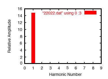
Fourier analysis of the sine wave input
Notice the extremely small harmonic and DC components of this sinusoidal waveform in the table above, though, too small to show on the harmonic plot above.
Ideally, there would be nothing but the fundamental frequency showing (being a perfect sine wave), but our Fourier analysis figures aren’t perfect because SPICE doesn’t have the luxury of sampling a waveform of infinite duration. Next, we’ll compare this with the Fourier analysis of the half-wave “rectified” voltage across the load resistor: (Figure below)
fourier components of transient response v(2)
dc component =   4.456E+00
harmonic  frequency   fourier    normalized   phase    normalized
no         (hz)      component   component    (deg)    phase (deg)
1        6.000E+01   7.000E+00     1.000000    -0.195       0.000
2        1.200E+02   3.016E+00     0.430849   -89.765     -89.570
3        1.800E+02   1.206E-01     0.017223  -168.005    -167.810
4        2.400E+02   5.149E-01     0.073556   -87.295     -87.100
5        3.000E+02   6.382E-02     0.009117  -152.790    -152.595
6        3.600E+02   1.727E-01     0.024676   -79.362     -79.167
7        4.200E+02   4.492E-02     0.006417  -132.420    -132.224
8        4.800E+02   7.493E-02     0.010703   -61.479     -61.284
9        5.400E+02   4.051E-02     0.005787  -115.085    -114.889
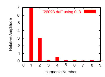
Fourier analysis half-wave output
Notice the relatively large even-multiple harmonics in this analysis. By cutting out half of our AC wave, we’ve introduced the equivalent of several higher-frequency sinusoidal (actually, cosine) waveforms into our circuit from the original, pure sine-wave.
Also take note of the large DC component: 4.456 volts. Because our AC voltage waveform has been “rectified” (only allowed to push in one direction across the load rather than back-and-forth), it behaves a lot more like DC.
Full-wave Rectification
Another method of AC/DC conversion is called full-wave (Figure below), which as you may have guessed utilizes the full cycle of AC power from the source, reversing the polarity of half the AC cycle to get electrons to flow through the load the same direction all the time.
I won’t bore you with details of exactly how this is done, but we can examine the waveform (Figure below) and its harmonic analysis through SPICE:
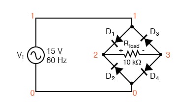
Full-wave rectifier circuit
fullwave bridge rectifier
v1 1 0 sin(0 15 60 0 0)
rload 2 3 10k
d1 1 2 mod1
d2 0 2 mod1
d3 3 1 mod1
d4 3 0 mod1
.model mod1 d
.tran .5m 17m
.plot tran v(1,0) v(2,3)
.four 60 v(2,3)
.end
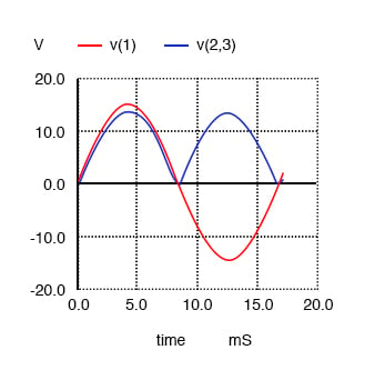
Waveforms for full-wave rectifier
fourier components of transient response v(2,3)
dc component =   8.273E+00
harmonic   frequency  fourier    normalized   phase   normalized
no         (hz)      component   component    (deg)   phase (deg)
1        6.000E+01   7.000E-02     1.000000   -93.519       0.000
2        1.200E+02   5.997E+00    85.669415   -90.230       3.289
3        1.800E+02   7.241E-02     1.034465   -93.787      -0.267
4        2.400E+02   1.013E+00    14.465161   -92.492       1.027
5        3.000E+02   7.364E-02     1.052023   -95.026      -1.507
6        3.600E+02   3.337E-01     4.767350  -100.271      -6.752
7        4.200E+02   7.496E-02     1.070827   -94.023      -0.504
8        4.800E+02   1.404E-01     2.006043  -118.839     -25.319
9        5.400E+02   7.457E-02     1.065240   -90.907       2.612
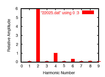
Fourier analysis of full-wave rectifier output
What a difference! According to SPICE’s Fourier transform, we have a 2nd harmonic component to this waveform that’s over 85 times the amplitude of the original AC source frequency!
The DC component of this wave shows up as being 8.273 volts (almost twice what is was for the half-wave rectifier circuit) while the second harmonic is almost 6 volts in amplitude. Notice all the other harmonics further on down the table.
The odd harmonics are actually stronger at some of the higher frequencies than they are at the lower frequencies, which is interesting.
As you can see, what may begin as a neat, simple AC sine-wave may end up as a complex mess of harmonics after passing through just a few electronic components.
While the complex mathematics behind all this Fourier transformation is not necessary for the beginning student of electric circuits to understand, it is of the utmost importance to realize the principles at work and to grasp the practical effects that harmonic signals may have on circuits.
The practical effects of harmonic frequencies in circuits will be explored in the last section of this chapter, but before we do that we’ll take a closer look at waveforms and their respective harmonics.
REVIEW:
- Any waveform at all, so long as it is repetitive, can be reduced to a series of sinusoidal waveforms added together. Different waveshapes consist of different blends of sine-wave harmonics.
- Rectification of AC to DC is a very common source of harmonics within industrial power systems.