How to Design a Capacitive Sensor for Liquid Level Measurements

Capacitive sensing is a widely used technique for liquid level measurement, based on detecting changes in capacitance caused by variations in the surrounding dielectric environment. Among the various capacitive sensing approaches, fringing field sensors are particularly well suited for non-contact liquid level detection, as their electric field extends beyond the sensor surface and can penetrate the wall of a non-metallic container.

By monitoring capacitance variations caused by changes in the liquid level, measurements can be performed without direct contact with the liquid. This characteristic makes the technology suitable for applications involving aggressive chemicals, sealed vessels, and hygienic or sterile systems.

This article describes the implementation of a fringing field capacitance sensor for liquid level measurement using the AnalogPAK IC. The design uses the device’s capacitive sensing resources to track changes in liquid level and employs the Math Core to calibrate the initial capacitance. This calibration compensates for sensor-to-sensor variation and environmental influences such as temperature, humidity, and material properties, helping improve measurement accuracy and stability.

A complete, ready-to-use design file is available. Engineers and enthusiasts can open the project, inspect the logic, and adapt the circuit using the free Go Configure Software Hub.

 

Circuit Connection

To understand the design, let’s first examine the connection diagram for the capacitance measurement application. Figure 1 shows the circuit where the capacitive sensor is charged through the 3 MΩ resistor R3 and discharged through the 300 Ω resistor R4. The SW1 button is used for the initial capacitance calibration. Resistors R5 and R6 are DNP and are used in cases where the max signal on the capacitive sensor exceeds a voltage higher than 1.6 V.

 

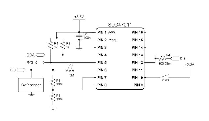
Figure 1. Circuit connection.

 

Fringing Field Capacitance Sensor for Liquid Level Measurement

A fringing field capacitive sensor uses the electric field extending beyond the edges of electrodes to detect changes in the dielectric constant of the surrounding environment. Unlike traditional parallel plate capacitors where the field is confined between plates, this sensor works based on coplanar interdigitated electrodes placed on a dielectric surface. When an alternating voltage is applied between the working and sensing electrodes, the electric field lines spread outward and penetrate the material near the electrodes. This penetration allows the sensor to measure properties such as the liquid level without direct contact. Figure 2 shows the structure of the fringing field capacitance sensor.

 

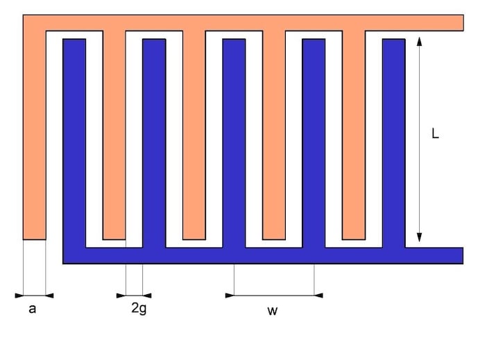
Figure 2. Configuration and geometry of the electrode used in fringing field capacitance sensors (blue is the sensing electrode and orange is the working electrode).

 

Figure 2 illustrates a coplanar interdigitated electrode sensor used for non-contact liquid level measurement. The sensor (see Figure 4) consists of equally spaced fingers on the working and sensing electrodes with gap (2g), finger length (L), width (α), and wavelength (w). It is placed against a dielectric sample of relative permittivity (ε_τ)and height (H). Electrodes are excited by potential +/- V, generating an electric field penetrating the dielectric, with maximum field penetration (h).

In addition to the configuration shown on Figure 2, there may be other possible designs of the 1-n-1 type, where n is the number of sensing electrodes. Some of the other possible configurations are shown in Figure 3.

 

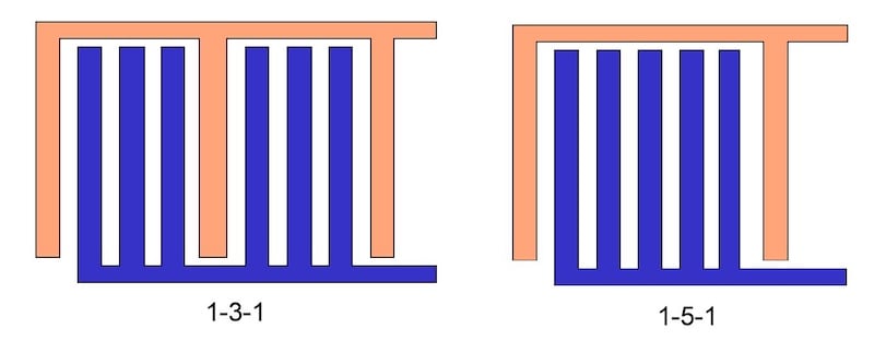
Figure 3. Possible electrode configuration for fringing field capacitance sensor

 

The operating principle is based on the fact that the capacitance between electrodes depends on the dielectric constant of the environment through which the electric field passes. As the liquid level rises near the sensor, more of the fringing field interacts with the liquid, which typically has a higher dielectric constant than air. This increases the effective capacitance. The relationship between capacitance and electrode geometry can be approximated by the equation:

 

$$C = \frac{2\varepsilon_r \varepsilon_0 L}{g\pi} \int_{\frac{(n-1)}{2}a + ng}^{\frac{(n-1)}{2}a + ng + a} \frac{1}{\sqrt{\left(\frac{x}{g}\right)^2 - 1}} \, dx$$

 

 

where: ε_τ = the relative permittivity of the liquid ε₀ = the permittivity of free space (usually air) L = the electrode length α = the electrode width g = the gap between electrodes

For an interdigitated structure with multiple fingers the penetration depth of the fringing field is given by:

 

$$h_n = g \sqrt{\left(n + \frac{(n+1)a}{2g}\right)^2 - 1}$$

 

From this equation, we can see that the penetration of the electric field mainly depends on the number of sensing electrodes.

As the liquid height H increases, the portion of the field passing through the liquid grows, but we also have a portion of the electric field passing through air. So, two capacitances are formed and the total capacitance equals the sum of the capacitance of the liquid level (C_H) and the capacitance of the air (C_A). Figure 4 shows the representation of this model where ε_τ and ε_l are the dielectric constants of the container wall and liquid, respectively. A simple representation of the total capacitance can be expressed as:

 

$$C_T = C_A + C_H$$

 

where:

 

$$C_A = \frac{2K\varepsilon_0(\varepsilon_r - 1)(H - L)}{\pi} \ln \left[ \sqrt{1 + \left(\frac{h_n}{g}\right)^2} + \frac{h_n}{g} \right]$$

 

$$C_H = \frac{2K\varepsilon_0(\varepsilon_r - \varepsilon_l)H}{\pi} \ln \left[ \sqrt{1 + \left(\frac{h_n}{g}\right)^2} + \frac{h_n}{g} \right]$$

 

$$K = \frac{N-1}{n+1}$$

 

where: N = total number of electrodes (working + sensing) n = number of electrodes between the two working electrodes

Using these equations, we can calculate the capacity changing due to liquid level changing. The relationship between liquid level and capacitance is nearly linear.

 

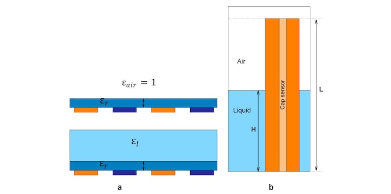
Figure 4. Representation of the splitting of a two-layered sensor

 

For this project this type of sensor was selected due to its advantages compared to other capacitance liquid level sensors.

First, fringing field sensors generate an electric field that penetrates deeply into the liquid even through the container wall. This allows the sensor to be mounted outside the container, which is not possible with conventional parallel plate or coaxial sensors.

Second, these sensors achieve high sensitivity even with compact dimensions. Parallel plate sensors require a much larger area to reach similar sensitivity. Additionally, the parameters of this sensor type can be easily calculated.

 

Design for Liquid Level Measurement

The operating principle of this design is based on the alternating charging and discharging of the capacitive liquid level sensor and measuring the changes in the time constant (τ). The design is shown in Figure 5.

 

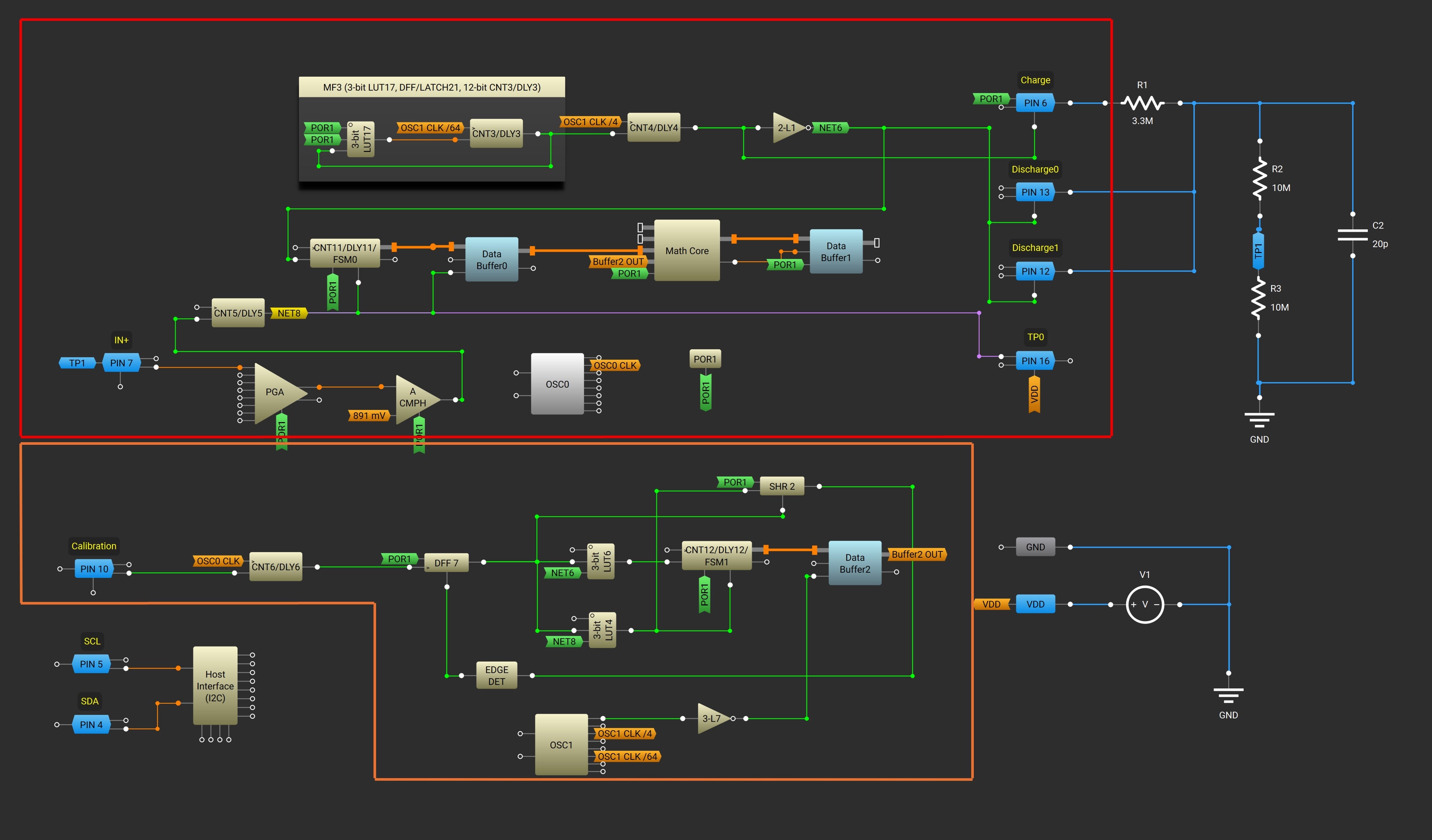
Figure 5. Design for liquid level measurement. (Click on image to enlarge)

 

It consists of two main parts:

The main part of the design (highlighted in red in Figure 5) implements the sequential charging and discharging cycles of the sensor and performs the capacitance measurement.

Let’s take a closer look at how this part works.

LUT7 and DLY3 form a frequency generator. Since the time constant measurement is performed only on the rising edge, DLY4 is used to introduce a delay on the falling edge. This increases the duration of the high-level signal, which increases the measurement frequency since we can save time on the duration of the low level. The signal generated is applied to the output pins configured in tri-state mode.

During charging, PIN6 outputs a high level, and the capacitive sensor is charged through a 3 MΩ resistor. PIN12 and PIN13 remain in a Hi-Z state during this process.

During discharging, PIN12 and PIN13 output a low level, and the sensor discharges through a 300 Ω resistor, while PIN6 switches to a Hi-Z state.

To measure the time constant, FSM0 is used. At the start of a new charging cycle, FSM0 is reset to its initial value and begins counting clock cycles. Since FSM0 operates from a 40 MHz oscillator, one counter increment corresponds to 25 ns.

The signal generated on the sensor during charging / discharging is fed to the PGA through PIN7. The PGA block configuration is shown in Figure 6. The signal from the PGA is then sent to the comparator. When the voltage reaches the threshold corresponding to the 1τ or 2τ, the comparator output switches to “0,” stopping FSM0 and triggering data storage into Buffer0 and Buffer1. The ACMP threshold can be adjusted via I²C by writing data to the 0x19E register. The threshold can range from 27 to 1620 mV with a 27 mV step.

The value from Buffer is then read and multiplied by 25 ns to convert it into the time constant. Since we know the resistor value, the sensor’s capacitance or its variation can be calculated.

The second part of the design (highlighted in orange in Figure 5) is used for calibrating the initial capacitance. The calibration works as follows: after the button connected to PIN10 is pressed, the output of DFF7 switches to a high level. DLY6 in this case acts as a filter, preventing false triggering from occurring.

When DFF7 is set to a high state, FSM1 operates in parallel with FSM0 during the next charging cycle of the capacitive sensor. The SHR2 block counts the number of completed charge-discharge cycles and after eight cycles, Buffer2 will be fully filled, and DFF7 will reset to its initial state. The averaged value stored in Buffer2 is subtracted from the measured value stored in Buffer0 in the Math Core.

 

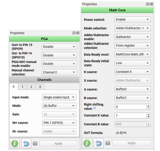
Figure 6. PGA and Math core configuration

 

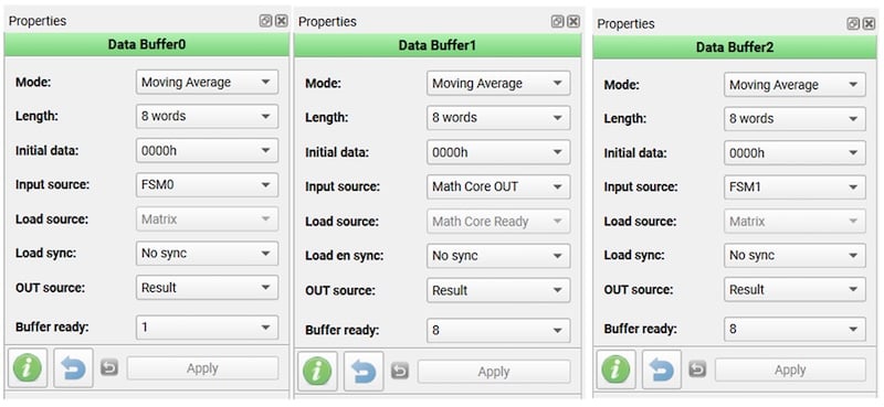
Figure 7. Data Buffer configuration

 

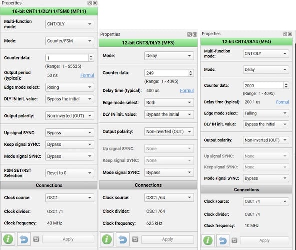
Figure 8. DLY 3, 4 and FSM configuration

 

Capacitive Liquid Level Sensor Demonstration Board

Figure 9 shows the schematic of the demo board. In this schematic, the SLG47011 performs the capacitance measurement function as described in Sections 2 and 4. Additionally, the board incorporates the IC, where one of its OPAMPs is configured as a buffer to monitor the signal from the capacitive sensor and reduce external interference during measurement.

 

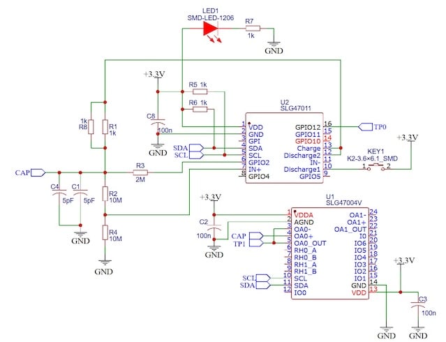
Figure 9. Schematic of the demonstration board

 

According to the schematic, a demonstration board was created for measuring the liquid level using a non-contact method. This board is shown in Figure 10 and Figure 11.

 

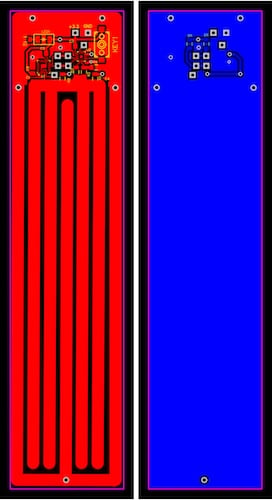
Figure 10. Demonstration board for measuring liquid level using the capacitive method.

 

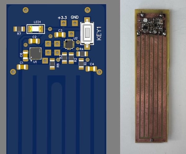
Figure 11. Test demo board

 

Test Results

The design was tested in hardware and the following waveform results were obtained: CH1 (yellow) – signal on the capacitive liquid level sensor. CH2 (blue) – output signal from the ACMP. The transition from LOW to HIGH occurs when the signal on the capacitive sensor reaches the threshold level at 1τ.

 

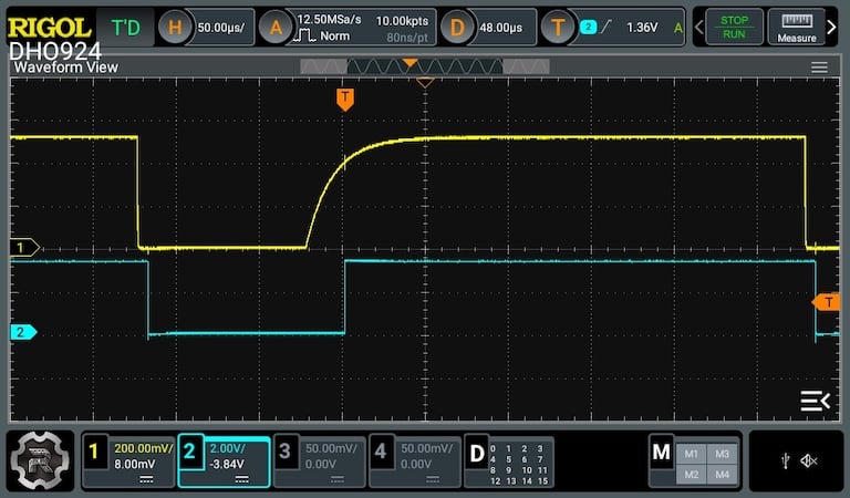
Figure 12. Discharging and charging cycle

 

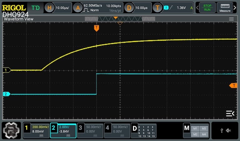
Figure 13. Zoomed charging

 

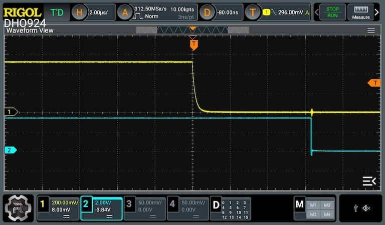
Figure 14. Zoomed discharging

 

Using the demonstration board described in Section 5, the following results were obtained.

Figure 15 shows a graph illustrating the dependence of the subtracted code from the AnalogPAK device on the liquid level height. In this graph, the orange line represents the data measured when the container is being filled, while the blue line represents the data when the container is being emptied. Each point on the graph corresponds to the averaged value of 100 measurements at a constant liquid level.

It is worth noting that the length of the sensor itself is 10 cm. From this graph, it can be seen that this dependence is almost linear across the entire range, which corresponds to theoretical expectations.

 

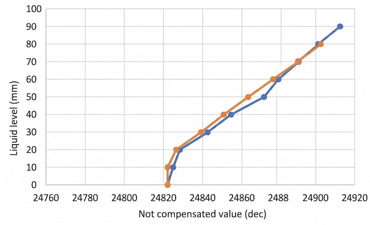
Figure 15. Dependency of read value from the SLG47011 which corresponds to capacity vs. liquid level. Orange line indicates container filling, blue indicates emptying

 

Issues and Limitations

The non-contact capacitive method for measuring the liquid level has both advantages and disadvantages. One of the major problems with this method is its high sensitivity to external signals and noise, which can lead to inaccurate measurements. This issue can be mitigated by taking a large number of measurements and taking the average as well as shielding the container with liquid.

This method also has limitations when measuring liquid levels in non-static containers. When the container is tilted, the amount of liquid within the sensor’s electric field decreases, causing measurement errors. To address this problem, multiple sensors can be placed on different walls of the container, or the sensor geometry can be designed to fit the specific shape of the container.

Additionally, capacitive sensors are sensitive to temperature changes, as the dielectric constant of the liquid used will vary with temperature. Under such conditions, measurement accuracy may decrease. To reduce this effect, additional temperature sensors can be used, and software algorithms can be implemented for temperature calibration.

Another problem is that this method cannot measure liquid levels through metal containers, since the electric field cannot penetrate metal materials.

 

A Practical Foundation

In this article we explored how to implement the design of a fringing field capacitive sensor for liquid level measurement using the SLG47011 AnalogPAK device. By measuring capacitance changes and applying baseline calibration, the system achieves stable and nearly linear liquid level detection across the sensor range.

The presented approach provides a practical foundation for capacitive level sensing applications, while highlighting the importance of sensor design, shielding, and environmental compensation for reliable measurements.

 

All images used courtesy of Renesas.