Facebook
 Google
 GitHub
 Linkedin
Adaptive Gain Control with the Least Mean Squares Algorithm
An introduction to the least mean squares algorithm and adaptive gain control through a simple example.
Here’s a cool trick you’ll literally never use unless you're using a microprocessor you bought for fractions of fractions of fractions of cents - heck maybe you'll even want to calculate how much some bulk quantity of these microcontrollers is per unit on your microcontroller, but you can’t because it's so cheap it can’t even do division. This division method is an introduction to adapative gain control with the least means square algorithm which I think will shed light on the workings of how it the iterative process calculates desired gains. Take a look at the following Matlab code which will converge to the correct value you are trying to divide to (without using the division operator).
DivideBy = 5;
mu = .1;
DivideByFactor = 1;
ref = 1;
num_iter = 20
for n = 1:num_iter
	y(n) = DivideBy * DivideByFactor;
	y_mag = abs(y(n));
	err(n) = ref - y_mag;
	DivideByFactor_time(n) = DivideByFactor ;
	DivideByFactor = DivideByFactor +mu*err(n);
end
That’s it! Do division in 12 lines of code without the division operator. This algorithm is derived from an adaptive or automatic gain control algorithm (AGC) used to maintain a certain amplitude at a systems output despite changes in amplitude at the input of the system. For example, in an audio system the AGC might reduce the volume if the signal is getting too large and increase it if the signal is getting too small.
In the digital domain, the system diagram can be seen in Figure 1. Try to mentally follow how each iteration of the algorithm above moves samples around the loop.
.png)
Figure 1
AGC uses the Least Mean Squares (LMS) algorithm to update a weight, called DivideByFactor in this implementation. What this algorithm is attempting to do is minimize the error between the output (y(n)) and the reference which we set to one. The reference signal is set to one so that DivideBy * DivideByFactor = 1 once the algorithm converges. Whole books can be written on the topic of the LMS algorithm, so I’ll keep it short. The lower branch of the loop can be written as:
$$DivideByFactor(n) = DivideByFactor(n-1) + \mu (ref-y(n))$$
This line is basically taking smalls steps towards the number which minimizes the error term:
$$err(n) = ref-y(n)$$
It takes a step $$\mu$$ of the error off from the DivideByFactor (which we initially set at 1 before the iterative loop). With enough steps, this perfectly converges to 1/DivideBy minimizing the error term to zero in the process. Mu is only stable within a certain range which is beyond the scope of this article but I’ll provide references below if you’d like to look into it further. You can test out how the system behaves with different values of $$\mu$$ by changing the $$\mu$$ parameter in the code. By making $$\mu$$ smaller, you can see that it takes more iterations to converge to the DivideByFactor. If you make $$\mu$$ too large, you’ll see the DivideByFactor diverge and continually increase (not good).
You can watch the DivideByFactor converge to the desired value by including the following code which plots the DivideByFactor_time term against each iteration:
plot([1:num_iter], DivideByFactor_time)
hold on
plot([1:num_iter], 1/DivideBy, 'color' , 'r')
axis([0 num_iter -0.05 1])
grid on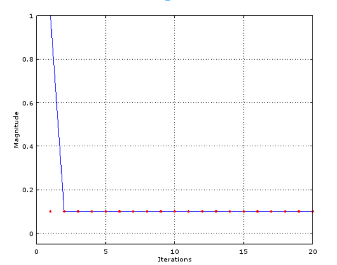
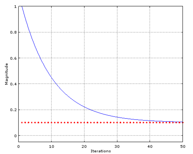
In this example, I’ve set DivideBy to 10 and plotted the DivideByFactor_time against each iteration. We expect it to converge to 0.10 (the dotted red line) and we see that after a couple iterations it converges quite nicely to the desired value. If we set $$\mu$$ to something really small like 1/10 of its original value, we can see that it take much longer for the value to converge to the desired value
Try changing $$\mu$$ to something large yourself and note what happens (you may need to extend the x axis and y axis to watch its behavior). Also try plotting the err(n) against iterations to watch it converge to 0!
So that’s it - an iterative division algorithm based on automatic gain control. If you don’t have Matlab, try running this in Octave which is open source and almost exactly the same as the Matlab language (minus some functionality). If you don’t want to download Octave, try porting the codes above to your favorite language and include it in the comments below for others to play around with! Note that if you arn't getting the right values out you probably need to increase the number of iterations!
For further reading into the LMS algorithm, check this out.
Related Content