 Facebook
 Google
 GitHub
 Linkedin
An Introduction to the CORDIC Algorithm
CORDIC is a hardware-efficient iterative method which uses rotations to calculate a wide range of elementary functions.
CORDIC (coordinate rotation digital computer) is a hardware-efficient iterative method which uses rotations to calculate a wide range of elementary functions.
This article reviews the basics of this algorithm and later demonstrates how we can use CORDIC to calculate the sine and cosine of a given angle.
Rotate to Perform a Wide Range of Operations
For the time being, let's forget about electronics and go back to high-school mathematics to see which operations can be achieved by simply rotating a vector.
Suppose that we have an efficient system that receives a vector and rotates it by an arbitrary angle $$\theta$$. Choosing the origin as the center of rotation, we will get to the point ($$x_1, y_1$$) by rotating the point ($$x_0, y_0$$) by $$\theta$$
$$x_R = x_{in} cos(\theta) - y_{in} sin(\theta)$$
$$y_R = x_{in} sin(\theta) + y_{in} cos(\theta)$$
Equation 1.
Figure 1 illustrates this rotation below.
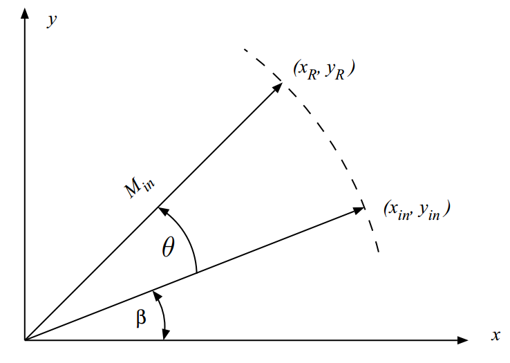
Figure 1. Rotating the input vector by $$\theta$$. Image courtesy of UCLA (PDF).
If we choose $$y_{in}=0$$ and $$x_{in}=1$$, after rotation we will have
$$x_R = cos(\theta)$$
$$y_R = sin(\theta)$$
Equation 2.
Therefore, we can simply calculate sine and cosine of an arbitrary angle through rotation.
For another example of the functions that can be calculated from rotation, consider the vector magnitude, $$\sqrt{x_{in}^2 + y_{in}^2}$$. To achieve this, we only need to rotate the input vector so that it is aligned with the x-axis. In this way, $$y_{R}=0$$ and the x component will give the vector magnitude.
Interestingly, the list of the functions that can be calculated from rotation is relatively long. Inverse trigonometric functions such as arctan, arcsin, arccos, hyperbolic and logarithmic functions, polar to rectangular transform, Cartesian to polar transform, multiplication, and division are some of the most important operations that can be obtained from variants of rotation.
The CORDIC algorithm attempts to provide a hardware-efficient method for calculating these functions. “Hardware-efficient” means that the algorithm avoids the use of multipliers and relies on only shifts and additions/subtractions. Note that other methods of implementing these functions, such as utilizing power series, usually need dedicated multipliers.
The Basics of CORDIC
Equation 1 can be simplified to:
$$\begin{bmatrix} x_{R} \\ y_{R} \end{bmatrix} = cos(\theta) \begin{bmatrix} 1 & -tan(\theta) \\ tan(\theta) & 1 \end{bmatrix} \begin{bmatrix} x_{in} \\ y_{in} \end{bmatrix} $$
Equation 3.
The above equation shows that for one rotation, we need to perform 4 multiplications (plus some additions/subtractions). The question that remains is, How can we avoid these multiplications?
The CORDIC algorithm resorts to two fundamental ideas to achieve rotation without multiplication. The first fundamental idea is that rotating the input vector by an arbitrary angle $$\theta_{d}$$ is equal to rotating the vector by several smaller angles, $$\theta_{i}$$, $$i=0, 1, \dots, n$$, provided $$\theta_{d} = \sum_{i=0}^{n} \theta_{i}$$. For example, a rotation of $$57.535˚$$ is the same as three successive rotations by $$45˚$$, $$26.565˚$$, and $$-14.03˚$$ (note that we can use negative angles too).
The second fundamental idea is that we can choose the small elementary angles in a way that $$tan(\theta_{i}) = 2^{-i}$$ for $$i=0, 1, \dots , n$$. In this way, multiplication by $$\tan(\theta_{i})$$ can be achieved by a bitwise shift which is a much faster operation compared to multiplication. You may wonder if, for a given $$\theta_{d}$$, we can satisfy the conditions of these two fundamental ideas simultaneously, i.e. $$\theta_{d} = \sum_{i=0}^{n} \theta_{i}$$ while $$tan(\theta_{i}) = 2^{-i}$$.
Note that, in practice, we face a limited accuracy and the convergence of these equations is important. Fortunately, the equations converge and by increasing $$n$$, we can increase the accuracy of calculations.
Choosing angles such that $$tan(\theta)$$ is an inverse power of two will allow us to perform these multiplications using bit shifts, but we still need to perform two other multiplications by $$cos(\theta)$$. Note that the multiplications by $$cos(\theta)$$ act as a system gain (because both the x and y components need to be multiplied by the same scaling factor). If we ignore this scaling factor, the rotation angle will be correct but we still have to scale down both the x and y components to arrive at the final values of $$x_R$$ and $$y_R$$. This is illustrated in Figure 2 where multiplications by $$cos(\theta)$$ are not applied and, as a result, $$x_R \prime$$ and $$y_R \prime$$ are achieved which are $$\frac{1}{cos(\theta)}$$ times larger than $$x_R$$ and $$y_R$$, respectively.
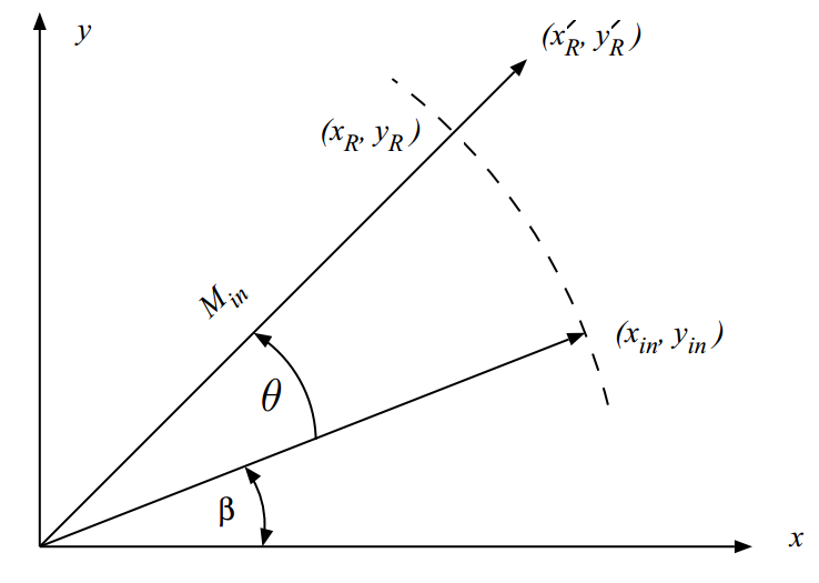
Figure 2. Multiplication by cos(θ) acts as a scaling factor.
Now let's examine the effect of this scaling factor when applying the successive elementary rotations of the CORDIC algorithm. Suppose that we want to rotate the input vector by $$57.535˚$$ which is $$45˚+26.565˚-14.03˚$$. The first rotation by $$45˚$$ will give us:
$$\begin{bmatrix} x_{0} \\ y_{0} \end{bmatrix} = cos(45˚) \begin{bmatrix} 1 & -1 \\ 1 & 1 \end{bmatrix} \begin{bmatrix} x_{in} \\ y_{in} \end{bmatrix} $$
Equation 4.
For the second rotation, we obtain:
$$\begin{bmatrix} x_{1} \\ y_{1} \end{bmatrix} = cos(26.565˚) \begin{bmatrix} 1 & -2^{-1} \\ 2^{-1} & 1 \end{bmatrix} \begin{bmatrix} x_{0} \\ y_{0} \end{bmatrix} $$
Equation 5.
Substituting Equation 4 into Equation 5 gives us:
$$\begin{bmatrix} x_{1} \\ y_{1} \end{bmatrix} = cos(45˚) cos(26.565˚) \begin{bmatrix} 1 & -1 \\ 1 & 1 \end{bmatrix} \begin{bmatrix} 1 & -2^{-1} \\ 2^{-1} & 1 \end{bmatrix} \begin{bmatrix} x_{in} \\ y_{in} \end{bmatrix} $$
Equation 6.
For the third rotation, we will have:
$$\begin{bmatrix} x_{2} \\ y_{2} \end{bmatrix} = cos(-14.03˚) \begin{bmatrix} 1 & 2^{-2} \\ -2^{-2} & 1 \end{bmatrix} \begin{bmatrix} x_{1} \\ y_{1} \end{bmatrix} $$
Equation 7.
Finally, we obtain:
$$\begin{bmatrix} x_{2} \\ y_{2} \end{bmatrix} = cos(45˚) cos(26.565˚) cos(-14.03˚) \begin{bmatrix} 1 & -1 \\ 1 & 1 \end{bmatrix} \begin{bmatrix} 1 & -2^{-1} \\ 2^{-1} & 1 \end{bmatrix} \begin{bmatrix} 1 & 2^{-2} \\ -2^{-2} & 1 \end{bmatrix} \begin{bmatrix} x_{in} \\ y_{in} \end{bmatrix} $$
Equation 8.
Equation 8 has two implications. First, each rotation mandates a scaling factor which appears in the final calculations. This means that it is possible to ignore the $$cos( \theta )$$ term of equation (3) and take the scaling factor into account at the end of the algorithm. Second, as we proceed with the algorithm, the angle of rotation rapidly becomes smaller and smaller. Hence, $$cos( \theta )$$ tends toward unity.
For example, with $$i=6$$, $$\theta_{i}$$ becomes $$0.895˚$$ which leads to a scaling factor of $$cos(0.895˚) = 0.99987$$. As a result, if the algorithm is designed to have more than six iterations, looking at the four significant figures, we obtain the following scaling factor:
$$K \approx cos(45˚) cos(26.565˚) \times \dots \times cos(0.895˚) = 0.6072$$
In summary, we can ignore the $$cos( \theta )$$ term of Equation 3 and apply a scaling factor of approximately $$0.6072$$ at the end of the process regardless of the desired rotation angle. For a more demanding application where higher accuracy is required, you can consider more significant figures for the scaling factor. This generally comes at no cost because, as explained in the example at the end of the article, the scaling factor is usually stored as an initial value in the system.
We can use a constant scaling factor because the algorithm uses some predefined angles in each elementary rotation. You may wonder if we still need a multiplier to take the scaling factor into account. As discussed later, we will see that we can sometimes apply the scaling factor somewhere else in the system without using a multiplier.
Therefore, omitting the scaling factor term from Equation 3, we obtain the following equations for the CORDIC algorithm:
$$x \left [ i+1 \right ] = x \left [ i \right ] - \sigma_{i} 2^{-i} y \left [ i \right ] $$
$$y \left [ i+1 \right ] = y \left [ i \right ] + \sigma_{i} 2^{-i} x \left [ i \right ]$$
Equation 9.
where $$\sigma_{i} \in \left \{ +1, -1 \right \}$$ determines the sign of the elementary angle and will be discussed in the next section of the article. The above equation shows that the algorithm will always perform a certain number of rotations with the predefined angles (for example, 12 rotations), and the only thing that the algorithm determines is whether each rotation will go clockwise or counter-clockwise during each iteration (choose $$\sigma_{i}$$ equal to +1 or -1).
Negative Feedback Mechanism of CORDIC
Equation 9 allows us to rotate a vector by some predefined angles without multiplication but how can we rotate the vector by an arbitrary angle? In other words, how should we choose the value of $$\sigma_{i}$$ for each iteration of the algorithm? This is accomplished by simply recording the angle of previous rotations and comparing the overall achieved rotation with the desired angle.
If the desired rotation is larger (smaller) than previously achieved rotation, then we need to rotate counter-clockwise (clockwise) in the next iteration. For example, assume we want a rotation of $$58˚$$. At the beginning of the algorithm, we have achieved zero rotation and $$58˚ > 0$$, so $$\sigma_{0}=1$$. This will bring about a rotation of $$45˚$$. In the second iteration, we see that the achieved rotation is still smaller than the target angle ($$58˚ > 45˚$$), so $$\sigma_{1}=1$$.
This will lead to a $$26.565˚$$ rotation in this iteration. Since $$58˚ < 45˚+26.565˚$$, the next iteration will choose $$\sigma_{2}=-1$$ which means that a rotation of $$14.03˚$$ will be applied clockwise and the overall rotation will be $$45˚+26.565˚-14.03˚=57.535˚$$. This process will go on until all the $$n$$ iterations of the algorithm are performed.
The described procedure is actually a negative feedback mechanism which computes the overall rotation and compares that to a reference value and chooses the new rotations in a way that minimizes the error signal ( $$\theta_{error} = \theta_d - \sum_{i=0}^{n} \theta_{i}$$ ).
The above mechanism is taken into account by adding another equation to the set of expressions in Equation 9 as follows:
$$x \left [ i+1 \right ] = x \left [ i \right ] - \sigma_{i} 2^{-i} y \left [ i \right ] $$
$$y \left [ i+1 \right ] = y \left [ i \right ] + \sigma_{i} 2^{-i} x \left [ i \right ]$$
$$z \left [ i+1 \right ] = z \left [ i \right ] - \sigma_{i} tan^{-1} ( 2^{-i} ) $$
Equation 10.
This equation accumulates the angle of all the previous rotations and compares that with an initial value $$z \left [ 0 \right ]$$. For example, in the rotation by $$58˚$$, we must choose $$z \left [ 0 \right ] = 58˚$$ and consider the sign of $$z \left [ i+1 \right ]$$ to decide about the direction of the next rotation.
There are two points that need to be further clarified here: first, as you may have noticed, we have to know the angle of each iteration, $$tan^{-1} (2^{-i})$$. For example, if we design a twelve-iteration algorithm, the value of the first twelve angles which satisfy $$tan (\theta_i) = 2^{-i}$$ should be stored in a lookup table (you can see this lookup table in Figure 3).
Second, the algorithm will perform the same number of iterations for any given $$\theta_d$$. For example, although $$57.535˚$$ is exactly equal to $$45˚+26.565˚-14.03˚$$, the algorithm will not stop with three iterations because this will require a different scaling factor (with three iterations $$K$$ will not be $$0.6072$$!). In this case, three iterations will lead to $$\theta_{error}=0$$ but the algorithm will continue until all the iterations are performed so that $$K$$ is $$0.6072$$ and $$\theta_{error}$$ is within the acceptable range.
The following figure shows the implementation of a single iteration in the CORDIC algorithm:
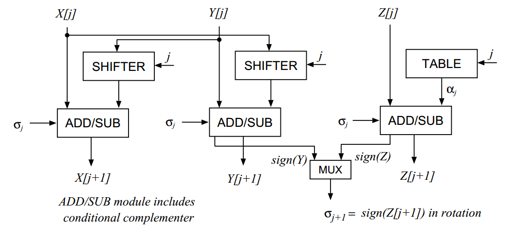
Figure 3. Implementation of Equation 9 for one iteration. Image courtesy of UCLA (PDF).
A Numerical Example
As an example, we will apply the CORDIC algorithm to calculate the sine and cosine of $$70˚$$ with $$n=12$$ iterations. As previously mentioned, to calculate the sine and cosine with rotation, we have to choose $$x_{in}=1$$ and $$y_{in}=0$$. The following table shows how the set of expressions in Equation 10 are evaluated for this example:
| Iteration ($$i$$) | $$\sigma_{i}$$ | $$x \left [ i \right ] $$ | $$y\left [ i \right ]$$ | $$z\left [ i \right ]$$ |
| - | - | $$1$$ | $$0$$ | $$70˚$$ |
| $$0$$ | $$1$$ | $$1$$ | $$1$$ | $$25˚$$ |
| $$1$$ | $$1$$ | $$0.5$$ | $$1.5$$ | $$-1.5651˚$$ |
| $$2$$ | $$-1$$ | $$0.875$$ | $$1.375$$ | $$12.4711˚$$ |
| $$3$$ | $$1$$ | $$0.7031$$ | $$1.4844$$ | $$5.3461˚$$ |
| $$4$$ | $$1$$ | $$0.6103$$ | $$1.5283$$ | $$1.7698˚$$ |
| $$5$$ | $$1$$ | $$0.5625$$ | $$1.5474$$ | $$-0.0201˚$$ |
| $$6$$ | $$-1$$ | $$0.5867$$ | $$1.5386$$ | $$0.8751˚$$ |
| $$7$$ | $$1$$ | $$0.5747$$ | $$1.5432$$ | $$0.4275˚$$ |
| $$8$$ | $$1$$ | $$0.5687$$ | $$1.5454$$ | $$0.2037˚$$ |
| $$9$$ | $$1$$ | $$0.5657$$ | $$1.5465$$ | $$0.0918˚$$ |
| $$10$$ | $$1$$ | $$0.5642$$ | $$1.5471$$ | $$0.0358˚$$ |
| $$11$$ | $$1$$ | $$0.5634$$ | $$1.5474$$ | $$0.0078˚$$ |
| $$11$$ | $$1$$ | $$0.5630$$ | $$1.5475$$ | $$-0.0062˚$$ |
Now we can take the scaling factor into account: $$x_{R} = 0.6072 \times 0.563=0.3419$$ which is pretty close to the $$cos(70˚)=0.342$$. The y component gives the sine of $$70˚$$ equal to $$y_{R} = 0.6072 \times 1.5475=0.9396$$ which is a very good approximation of $$sin(70˚)=0.9397$$.
As mentioned previously, we can sometimes avoid multiplication by the scaling factor. This is possible in the above example. To this end, we can apply the scaling factor to the initial values and start from $$x_{in} = 0.6072$$ and $$y_{in} = 0$$ so that the final multiplication is omitted. In other words, since the initial values are constants, the application of the scaling factor merely changes the constants that are used.
Featured image used courtesy of HP Museum.
Related Content


Took me a few months to completely understand, but whooo, finally got it! I’ll sleep 5% better now. By far the best material on CORDIC. Thanks man!
Links:
https://en.wikipedia.org/wiki/CORDIC
https://ru.wikipedia.org/wiki/CORDIC
https://de.wikipedia.org/wiki/CORDIC
http://cordic-bibliography.blogspot.de/p/what-is-cordic.html
Best explanation so far. Thank you so much