Analyzing Oscillator Frequency in an LTspice Negative Voltage Charge Pump

To begin with, let's introduce the schematic shown in Figure 1, which shows you the LTspice version of a circuit that uses two capacitors, four switches, and one square wave to achieve voltage inversion. This will be the example schematic used throughout this article.

 

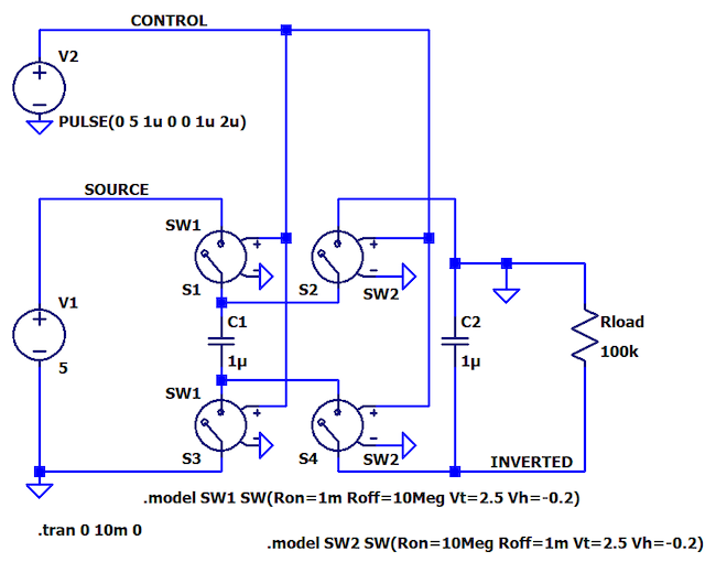
Figure 1. An LTspice circuit uses two capacitors, four switches, and a square wave to achieve voltage inversion.

 

Next, before looking too much further at this figure and our overall subject, let’s briefly review some key takeaways from previous articles:

• The inverted voltage is unregulated. It can function as a power supply, but the output voltage will decrease as the load current increases.
• The output voltage will be less sensitive to load current if we take measures to reduce the effective output resistance.
• Simulations help us to determine whether the circuit can provide adequate output-voltage magnitude at a given load current.
• The circuit’s charge/discharge cycle results in output ripple at f_OSC—i.e., the frequency of the square wave that controls the switches.
• We can reduce output ripple by choosing a low-ESR output capacitor, increasing output capacitance, or passing the output voltage through a linear regulator.  

Thus far, I’ve been using an oscillator frequency of 500 kHz. You may have been wondering how I arrived at this number. Why not 50 kHz? Or 5 MHz? In this article, we’ll focus on the role of oscillator frequency in the system and discuss the pros and cons of increasing or decreasing f_OSC.

 

The Initial Oscillator Frequency—Use the LTspice .param Feature

A good place to start is somewhere between 100 kHz and 1 MHz. My intuition tells me that these are reasonable frequencies for this type of application, but also, I know that inductor-based switchers often operate in this range.

In any case, changing frequencies is easy when you’re working with simulations, so there’s no need to worry too much about the initial frequency. As long as you start with a frequency that gives you an accurate representation of the circuit’s basic functionality, you can effectively begin the optimization process that will lead to an appropriate frequency for a given application.

By the way, changing frequencies is even easier if you make use of LTspice’s .param feature (Figure 2).

 

Figure 2. Section of the schematic in Figure 1 shows the .param feature in LTspice.

 

Here I have a .param statement where I define the oscillator frequency (Fosc). The logic-high duration (Ton) and the period are calculated from Fosc, and I use the Ton and Period parameters in the fields for the PULSE component (don’t forget the curly brackets!). This handy trick can save quite a bit of time, plus it’s helpful to see the frequency right there on the schematic. I typically think in terms of frequency, not period, and for me, trying to repeatedly decode something like PULSE(0 5 1u 0 0 0.68u 1.36u) into frequency is a bit tiresome.

 

Frequency and Energy of a Negative Voltage Charge Pump

The basic phenomenon that informs frequency optimization is energy. In physical systems, the general rule is that higher frequencies correspond to higher energy. This intuitively makes sense if we remember that movement is directly associated with energy—more specifically, kinetic energy. If you turn a light switch on and off, you’re expending energy as your finger moves. If you flip the switch more frequently—and don’t change anything else—you must produce more finger movement in the same amount of time; thus, you’re expending more energy per unit of time, which is the scientific definition of power. Similarly, the “movement” of a voltage between 5 V and ground involves the use of energy, and if that voltage transition occurs more frequently, more energy per unit of time is required.

The oscillator in the negative voltage charge pump is the fundamental source of energy for the inversion that occurs. Actually, if you look back at the SPICE schematic that I designed, the oscillator is situated above the other components, with its output distributed to all four switches as though it’s a power supply. That’s how I think of the oscillator in a system like this. Basically, it uses voltage “motion” to transfer and distribute energy that efficiently accomplishes the work of pulling the input voltage beyond the ground and into the negative voltage region.

 

Switched-capacitor Circuit Frequency Pros and Cons

If f_OSC is too low, the switching system is starved for power, and this is manifested as a reduced ability to supply load current—in other words, as higher output resistance. In fact, the output resistance of an idealized switched-capacitor circuit is inversely proportional to oscillator frequency (and to the value of C1). “Idealized,” in this case, means that we’re ignoring the resistance of the switching elements and the equivalent series resistance (ESR) of the capacitors.  

 

$$R_{OUT}\approx\frac{1}{C_1f_{OSC}}$$

 

From here, you can see the relationship between f_OSC and R_OUT in the plot below in Figure 3.

 

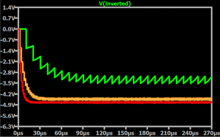
Figure 3. Plot showing the relationship between f_OSC and R_OUT.

 

With low load resistance, the steady-state output-voltage magnitude decreases significantly as oscillator frequency decreases.

In the figure, the different colors represent:

• Green trace = 100 kHz
• Beige trace = 500 kHz
• Red trace = 1 MHz

Also, for this simulation, C1 = 1 μF and C2 = 3 μF.

If f_OSC is too high, the switching system has access to more energy than it needs, and the overall circuit dissipates more power just to sustain the operation. Higher frequencies are also more likely to generate problematic electromagnetic interference (EMI).

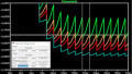
You can reduce output ripple by raising the oscillator frequency (Figure 4).

 

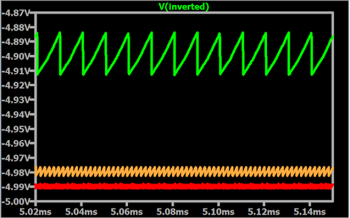
Figure 4. Plot showing ripple magnitude for three different frequencies.

 

The plot above shows the ripple magnitude for the same circuit with three different oscillator frequencies.

• Green trace = 100 kHz
• Beige trace = 500 kHz
• Red trace = 1 MHz

Also, for this simulation, C1 = 1 μF and C2 = 3 μF.

This is a worthwhile technique if you really need to minimize ripple, but before you take any action, it’s important to truly understand your system’s power-supply requirements. Ripple that looks terrible on a zoomed-in scope display may have no meaningful effect on the performance of components that are powered by that ripply voltage, and you don’t want to reduce efficiency or exacerbate EMI issues just to reduce ripple that isn’t actually impairing operation. 

All said and done, choosing an oscillator frequency for a switching power supply is a balancing act. Simulations can help you optimize your design, and you might consider building a prototype with a variable-frequency oscillator. In any event, keep the basic trade-off in mind: higher frequencies favor performance—i.e., lower output resistance and lower ripple—and lower frequencies extend battery life.