 Facebook
 Google
 GitHub
 Linkedin
Image Arithmetic in DSP: Image Averaging and Image Subtraction
Learn how to employ arithmetic operations on images as a way to enhance image quality, detect changes, and reduce noise.
In digital image processing, we can use arithmetic operations to enhance a given image or extract some useful information.
In this article, we’ll look at two of these operations: image addition (averaging) and image subtraction.
While image averaging is usually utilized for noise reduction, image subtraction can be employed to mitigate the effect of uneven illuminance. Moreover, we’ll see that image subtraction allows us to compare images and detect changes.
This makes image subtraction a fundamental operation in many motion detection algorithms.
Digital Image Processing Using Point Operations
In a previous article, we discussed point operations in digital image processing. There, we discussed the fact that a digital image can be described by a two-dimensional array of small elements called pixels.
A grayscale image can be represented by a two-dimensional function I[x, y] where the arguments x and y are the plane coordinates that specify a particular pixel of the image. The value of the function determines the intensity or gray level of the image at that point.
The addition operation between two images I1[x, y] and I2[x, y] is represented by:
S[x, y] = I1[x, y] + I2[x, y]
Note that the corresponding pixels of the two images are added together to create the output pixel value at the same pixel location.
Now, let's discuss how we can use the addition operation to add two different images together and create nice effects in photographs.
Image Averaging for Noise Reduction
One of the more interesting applications of the image averaging (or image addition) operation is suppressing the noise component of images.
In this case, the addition operation is used to take the average of several noisy images that are obtained from a given input image. Assume that our desired input image is I[x, y]. The imaging process and the quantization operation of the utilized A/D converter lead to a noisy image Inoisy[x, y].
Assume that the noise effect can be modeled as a noise image, n[x, y], that is added to the noise-free input I[x, y]. This gives us
Inoisy[x, y]= I[x, y] + n[x, y]
If we capture the same input image several times, the noise-free image I[x, y] will remain the same while the noise component will vary from one capture to the other. If we assume that the noise components are not correlated with each other and the mean value of the noise is zero, then averaging several noisy images should suppress the noise. This is due to the fact that I[x, y] is the same from one capture to the other and is not suppressed by averaging.
However, the noise image has random variations and approaches its mean value (zero) by taking the average.
Figure 1 shows a noisy image of the NGC 3749 galaxy.

Figure 1. Image adapted from Astronomy.com.
The noise has created bright spots that make it difficult to recognize the individual stars. If we capture this image many times and apply the averaging technique, the bright regions of noise will fade away and we’ll be able to more easily recognize the individual stars.
The result of averaging 500 images is shown in Figure 2.
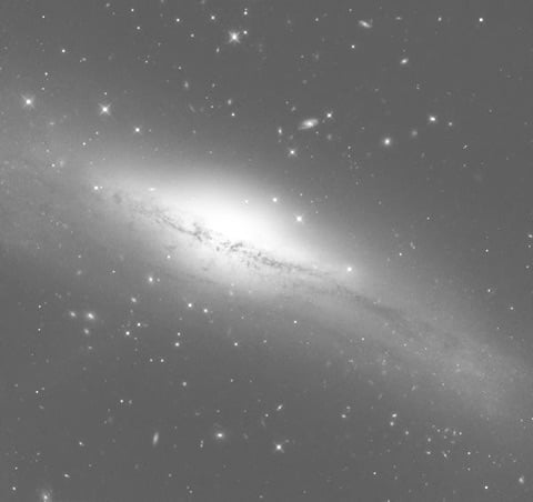
Figure 2. Image adapted from Astronomy.com.
It can be shown that averaging M noisy images reduces the noise variance by a factor of M. In other words, it increases the signal-to-noise ratio (SNR) by a factor of M.
It is worthwhile to mention that signal averaging is a general technique and finds use in other fields of electronics. For a detailed discussion of this technique, please refer to my article Use Signal Averaging to Increase the Accuracy of Your Measurements. Using this technique, we can measure a signal that is orders of magnitude smaller than the noise component, provided that the noise is not correlated with our desired signal and has a zero mean.
Image Subtraction
Subtraction of I2[x, y] from I1[x, y] is represented by:
D[x, y] = I1[x, y] - I2[x, y]
Note that the subtraction operation is performed on a point by point basis as well. This operation has several interesting applications, including correcting uneven illuminance and comparing images.
Image Subtraction for Correcting Uneven Illuminance
First, let's look at the application of the subtraction operation in mitigating the effect of uneven illuminance. As an example, consider the light microscope image of collenchyma cells shown in Figure 3.
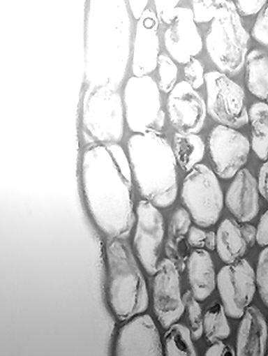
Figure 3. Image adapted from Siyavula.
As you can see, the top left corner of the image is much brighter than the rest of it.
To correct this undesired effect, we can create a reference image that has the same illumination variation. This can be achieved by capturing the image of a uniform scene (e.g. a white sheet of paper).
Such a reference image for the example of Figure 3 is shown in Figure 4.

Figure 4. A reference image with a corresponding level of illumination variation as seen in Figure 3
If we subtract this reference from the image in Figure 3, a relatively larger value will be subtracted from those regions that are strongly illuminated. This means that the pixel values of the brighter regions, such as the top left corner, will decrease much more than the pixel values in the weakly illuminated areas.
The subtraction operation can lead to negative pixel values in the difference image. If the negative values are not supported by our image format, we have to add a sufficiently large constant to the minuend image (the image in Figure 3) to avoid negative values in the difference image. However, adding this constant to the input image can lead to overflow because, in practice, we are using a limited number of bits to represent each pixel value.
Because of this, before adding the constant, we might need to change our data type to a larger type so as to avoid overflow. For example, while we usually use eight-bit data types to represent the pixel values of a grayscale image, we might need to use a 16-bit data type to successfully perform the calculations.
In this example, we add a constant of 109 to the minuend image and perform the subtraction (Figure 4 is subtracted from Figure 3 plus 109). The result is shown in Figure 5.
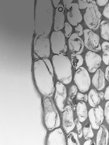
Figure 5
As you can see, this image has a much more uniform illumination.
Image Subtraction for Comparing Images
Another important application of the subtraction operation is finding differences between two images.
If the input images are the same at a given pixel location, they have the same value and the grayscale value of the difference image will be zero (black) at that location. However, the differences will lead to a non-zero output value and can be easily recognized.
Consider the example images shown in Figure 6.
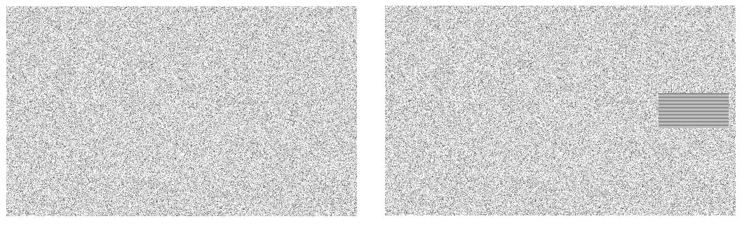
Figure 6
The two images are the same except that the image on the right side includes a hatched rectangular area. The difference image is shown in Figure 7.

Figure 7
As you can see, the non-zero pixels can be used to determine the differences between the inputs.
Applications in Motion Detection Algorithms
This simple observation is the basis for several motion detection algorithms. These algorithms capture a sequence of images from the same scene at different times and use the subtraction operator to detect changes.
It is worthwhile to mention that motion detection is a challenging problem and a wide variety of algorithms for different applications are discussed in the literature. If you're interested in this concept, you may consider referring to this article on advances in vision-based human motion capture and analysis.
In practice, the similar regions of the images that are compared by the subtraction operation may not have exactly the same grayscale value. For example, the illumination variation from one capture to the other can lead to slightly different pixel values even in similar regions. Therefore, we might need to find an appropriate threshold value in order to determine whether or not a given output pixel value represents a difference between the input images.
Conclusion
In this article, we looked at two important arithmetic operations: image addition and image subtraction. The addition operation can be used to suppress the noise component and increase the SNR. Two important applications of the subtraction operation are mitigating the effect of uneven illuminance and finding differences between images. The change detection feature of the subtraction operation makes it very useful in many motion detection algorithms.
To see a complete list of my articles, please visit this page.


So what would be the best way to see very faint differences in light level between pixels? Something like super amplification. I know this would result in many areas going to white (in a mono image). But there is probably a way to blank that out. BTW, I have found a free program called FIJI that has an easy to use GUI interface with great image calculators in it’s many menu choices. This is a quick way to try out different calculations.