Facebook
 Google
 GitHub
 Linkedin
Companding: Logarithmic Laws, Implementation, and Consequences
This article aims to explain the logarithmic laws of companding and the methods of implementation along with the effects these methods bring into the PCM-based telephone systems.
This article aims to explain the logarithmic laws of companding and the methods of implementation along with the effects these methods bring into the PCM-based telephone systems.
Background study
Companding is a portmanteau for a “compressing-expanding” mechanism. It compresses the signals before transmitting on a band-limited channel and expands them when received. During compression, an analog signal is quantized to create a digital signal using unequal steps in order to amplify the quiet sounds while attenuating the loud ones. Conversely, at the receiver, the digital signal is converted back to an analog signal after expansion, in which the low amplitude signals are amplified less when compared to higher ones.
This act would alter the dynamic range of the signal, facilitating the transmission of a signal with a large dynamic range over a channel with smaller dynamic range.
Companding in PCM based digital telephone systems
Human speech is composed of different amplitude utterances and sounds called phonemes, and possesses a large dynamic range. However, the required bandwidth to be transmitted over in PCM-based telephone networks is around 4 KHz, making companding a good fit in this situation.
Logarithmic Companding Curves
In companding, quantization intervals increase logarithmically with an increase in the amplitude of the signal. Two such logarithmic companding curves are A-law curve and µ-law curve, which differ in the slope at their origins, as shown in Figure 1. These two encoding schemes are recommended by ITU Standardization Sector for Telecommunications (ITU-T) G.711 and are the international companding standards.
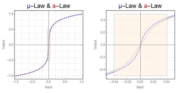
Figure 1: Graphic shows µ-Law and a-Law over the entire range (left) and zoomed into the highlighted region (right). Image by Mark Hughes, AAC.
A-Law
European countries practice A-Law companding. The mathematical expression for A-law compression in continuous domain (PDF) is given as:
$$ F(x)=\frac{sgn(x)}{1+ln(A)}\left \{ \begin{matrix}
A\;|x| & 0 \leq|x|\leq\frac{1}{A}\\
1+ln(A|x|)& \frac{1}{A}\leq |x|\leq 1
\end{matrix}\right.$$
where:
x is the input signal
sgn(x) is the sign of the input signal
|x| is the absolute value of x
A = 87.6 is the compression parameter defined by Consultative Committee for International Telephony And Telegraphy (CCITT) G.711
The corresponding A-law expansion equation (PDF) is:
$$ F^{-1}(y)=sgn(y)\left \{ \begin{matrix}
\frac{|y|\left[1+ln\left(A\right)\right]}{A} & 0 \leq|y|\leq\frac{1}{1+ln\left(A\right)}\\
\frac{exp\left(|y|\left[1+ln\left(A\right)\right]-1\right)}{A+A\left[ln\left(A\right)\right]} & \frac{1}{1+ln\left(A\right)}\leq |y|\leq 1
\end{matrix}\right. $$
where:
y is the companded signal
sgn(y) is the sign of the companded signal
|y| is the absolute value of y
A = 87.6 is the compression parameter defined by CCITT
µ-law
The µ-law companding technique is deployed in North America and Japan. The analog version of µ-law (PDF) is given as:
$$ F\left(x\right) = sgn(x)\frac{ln\left(1+\mu|x|\right)}{ln\left(1+\mu\right)} \qquad -1\leq x \leq 1 $$
... for compression
and
$$ F^{-1}\left(y\right) = sgn(y)\frac{\left(1+\mu\right)^{|y|}-1}{\mu} \qquad -1\leq y \leq 1 $$
... for expansion
where:
x is the input signal
y is the companded signal
sgn(x) is the sign of the input signal
sgn(y) is the sign of the companded signal
|x| is the absolute value of x
|y| is the absolute value of y
µ = 255 is the compression parameter defined by CCITT G.711
Piecewise linear approximation
Direct conversion of input data into logarithmic scale is troublesome from an implementation point of view. Due to this, the logarithmic curves of both A-law and µ-law are approximated using 16 straight line segments called chords, as shown in Figure 2 (piecewise linear approximation).
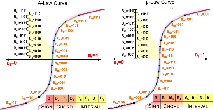
Figure 2: Piecewise linear approximation of A-law and µ-law curves. Image by Mark Hughes, AAC
Each of these chords, irrespective of length and slope, is then divided into 16 equal-spaced quantization intervals. However, the size of the quantization interval doubles from one chord to another as we move away from the origin. This is evident in Figure 3, where the quantization interval of the chord (n+1) is two times greater than that in the case of chord n. While this is true for all the chords of µ-law, A-law has an exception because two of its consecutive chords start from the origin (towards both the positive and negative side) and exhibit the same quantization interval.
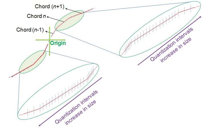
Figure 3: Uniform quantization of each chord resulting in an increase in the size of quantization intervals as we move away from the origin. Image by Sneha H. L., AAC.
Although both A-law and µ-law are approximated using the same number of chords, the same number and their slopes differ in both of them, as shown in Figure 4. This causes the quantization levels to differ from one law to another resulting in the variation of the digital value associated with a particular input level. Due to this, it is seen that A-law offers greater dynamic range than µ-law at the price of greater distortion at low amplitude signals.
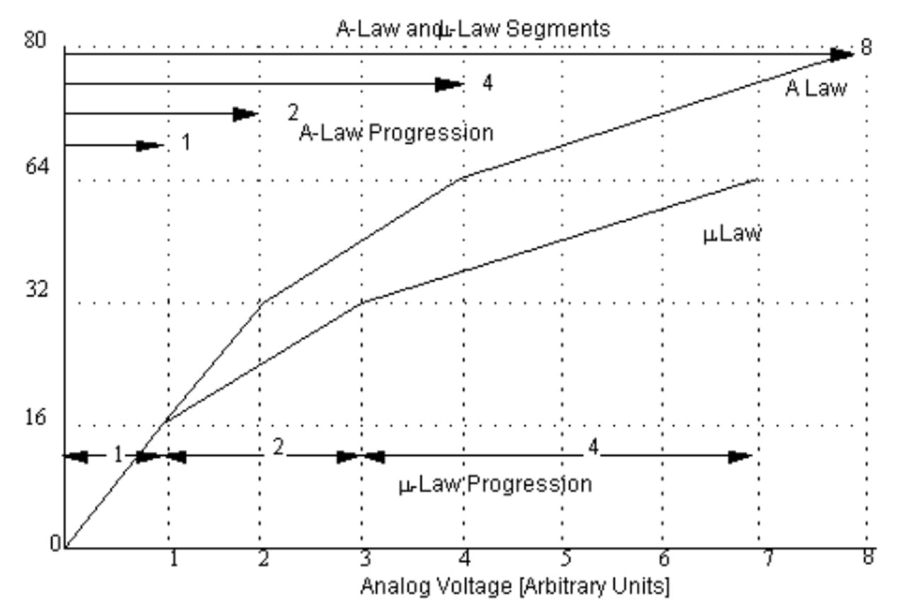
Figure 4: A-law and µ-law piecewise approximations differing in length and slopes of the chords. Image courtesy of www.jugandi.com.
Both of these laws convert 16-bit linear PCM signal (data) into 8-bit logarithmic data. Among these eight bits (shown as B1:8 in Figure 2), the first bit (B1) indicates the sign of the signal: positive or negative. The next three bits (B2:4) identify the chord and the last four bits (B5:8) indicate the exact position of the input signal within that particular chord.
Implementation
Companding can be implemented directly from the compression and expansion equations covered in the section “Logarithmic Companding Curves”. Here, each of the input sample is subjected to the compression equation and then uniformly quantized before transmission, after which the original signal is obtained back at the receiver using the corresponding equation for expansion (PDF).
However, instead of this computationally demanding technique, we can resort to a look-up table based methodology (PDF) to achieve companding. In the latter case, we design a table consisting of partition levels (used at the transmitter) and reconstruction levels (used at the receiver) using the respective compression and expansion equations. Once the table is complete, companding just becomes a matter of routing. This technique (PDF), although easy from a calculation point of view, proves to be memory-extensive.
At this stage, note that as µ-law companders (devices carrying out the process of companding) and A-law companders are incompatible, the µ-law companders must be linked with conversion circuits to establish interoperability.
Consequences of Companding
In companding, the rate of compression depends on the values of compression parameters µ and A of the equations presented in the section “Logarithmic Companding Curves”. Greater the value of compression parameters, higher is the rate of compression (Figure 5).
.jpg)
Figure 5: Compression curves for different values of compression parameters in (a) µ law (b) A law.
Higher compression rates imply greater non-linearity in quantization, which means there is a better representation of lower amplitude signals (using more number of bits) compared to higher amplitude ones. This indicates that, in a companded signal, the quantization error will be at its minimum at low levels and will gradually increase with an increase in the level of the input signal (PDF). In addition, the smaller the quantization interval, the better the signal-to-quantization noise ratio (SQNR). This means companding increases the SQNR at low-level signals while degrading it for higher amplitude ones (PDF).
The scenario well suits the demand for telephone systems which primarily transmit human speech wherein low amplitude quieter phonemes occur more frequently when compared to high amplitude louder phonemes (PDF). A direct consequence of this is an improvement in the quality of the audible signal, as we would have accounted for the sensitivity issues posed by the human ear.
Conclusion
This article explains the process and implementation of companding in PCM based telephone systems by adhering to logarithmic companding laws. Companding has brought about many positive impacts on systems, making it technologically meritorious.
Other References
Principles of Speech Coding
Authors Tokunbo Ogunfunmi, Madihally Narasimha
Illustrated Edition
Publisher CRC Press, 2010
ISBN 1439882541, 9781439882542
Related Content