 Facebook
 Google
 GitHub
 Linkedin
Hall Effect Current Sensing: Open-Loop and Closed-Loop Configurations
Learn the basics of Hall effect current sensors in this technical article.
Current sensors are widely used in a variety of applications. A common technique is resistive current sensing where the voltage drop across a shunt resistor is measured to determine the unknown current. Shunt resistor-based solutions do not provide galvanic isolation and are not power-efficient, especially when measuring large currents.
Another widely used technique is based on the Hall effect. A Hall effect current sensor provides a higher level of safety due to its galvanic isolation between the sensor and the current to be measured. It also avoids the sizable power dissipation of the shunt resistor employed in resistive current sensing methods.
In this article, we’ll take a look at the basics of Hall effect current sensors.
Open-Loop Current Sensing
The structure of a Hall effect-based open-loop current sensor is shown in Figure 1.
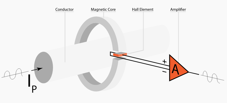
Figure 1. Image courtesy of Dewesoft
The current to be measured flows through a conductor that is inside a magnetic core. In this way, the current creates a magnetic field inside the core. This field is measured by a Hall effect sensor placed in the core air gap.
The output of the Hall sensor is a voltage proportional to the core magnetic field which is also proportional to the input current. The signal produced by the Hall device is usually processed by a signal conditioning circuitry. The signal conditioning circuitry can be a simple amplification stage or a more complicated circuit designed to eliminate the Hall device drift error, etc.
Why Do We Need a Magnetic Core?
Assume that there is no magnetic core. The magnetic field at a distance of r from an infinitely long, straight conductor that carries an electric current of I is given by:
\[B = \frac{µ_0I}{2\pi r} ~ , ~ µ_0 = 4\pi \times 10^{-7}\frac{H}{m}\]
where µ0 is the permeability of free space. For I=1 A, r=1 cm, we obtain:
\[B = 2 \times 10^{-5}~Tesla = 0.2~Gauss\]
To have a feeling about how small this magnetic field is, note that the earth’s magnetic field is about 0.5 Gauss. Hence, it is very challenging to measure a 1-A current by sensing the magnetic field it produces in free space. To combat this problem, we can use a magnetic core to confine and guide the magnetic field produced by the current. The core offers a path of high permeability for the magnetic field and acts as a field concentrator. The magnetic field inside the core can be hundreds or thousands of times larger than that a given current can produce in free space.
The Air Gap
As shown in Figure 1, the magnetic core is designed with an air gap in which the Hall sensor is placed. The air gap can lead to fringing flux phenomenon where some flux lines deviate from their straight path and hence, do not go through the sensor as expected. This fringing effect is shown in Figure 2.
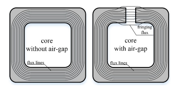
Figure 2. Image courtesy of R. Jez
Because of the fringing effect, the magnetic flux density sensed by the Hall device can be smaller than the magnetic flux density inside the core. In other words, the air gap can reduce the efficacy of the core at converting the primary current into a strong magnetic field. However, if the gap length is small compared to the gap cross-sectional area, the effect of the fringing effect can be relatively small.
We need the air gap to be able to measure the magnetic field inside the core. Besides, the air gap allows us to modify the overall reluctance of the core. Note that a high current can create a large magnetic field inside the core and saturate it. This can limit the maximum current that can be measured. Adjusting the air gap length, we can change the core saturation level. Figure 3 shows how the sensed magnetic flux density changes with the air gap length for a given core.
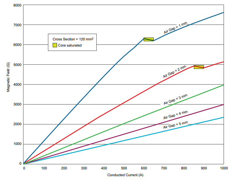
Figure 3. Image courtesy of Allegro
With smaller air gaps, we can achieve a larger magnetic gain (gauss-per-ampere gain). However, a smaller air gap can make the core saturate at a relatively smaller current. Hence, the gap length directly affects the maximum current that can be measured. In addition to the gap length, there are other factors, such as the core material, core dimensions, and core geometry, that determine the efficiency of a magnetic core. For more information about cores suitable for high-current applications (>200 A), please refer to this application note from Allegro.
Limitations of Open-Loop Current Sensing
With an open-loop configuration, non-ideal effects, such as linearity and gain errors, can affect the measurement accuracy. For example, if the sensitivity of the sensor changes with temperature, a temperature-dependent error will appear at the output. Besides, with open-loop current sensing, the core is subject to saturation. Moreover, the offset of the Hall sensor as well as the core coercivity can contribute to errors.
Closed-Loop Current Sensing
The closed-loop Hall effect current sensing technique is illustrated in Figure 4.
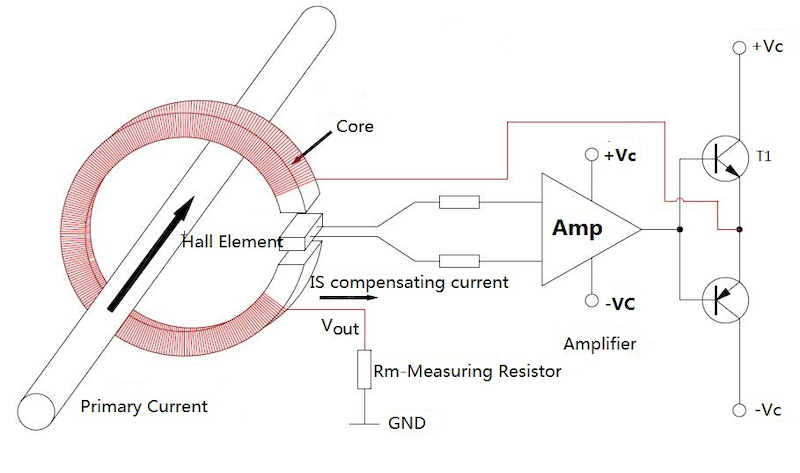
Figure 4. Image courtesy of Cheemi-Tech
As the name suggests, this technique is based on negative feedback concepts. In this case, there is a secondary winding that is driven by the output of the feedback path. The feedback path senses the magnetic field inside the core and adjusts the current through the secondary winding so that the total magnetic field of the core becomes equal to zero. Let’s see how this circuit works.
The current to be measured flows through the primary conductor and creates a magnetic field inside the core. This field is measured by a Hall effect sensor placed in the core air gap. The output of the Hall sensor, which is a voltage proportional to the core magnetic field, is amplified and converted to a current signal that goes through the secondary winding. The system is designed in a way that the current going through the secondary winding produces a magnetic field that opposes the magnetic field of the primary current. With the total magnetic field being equal to zero, we should have:
\[N_pI_p = N_sI_s\]
where Np and Ns are respectively the number of turns of the primary and secondary windings; and Ip and Is are the primary and secondary currents. In Figure 4, we have Np = 1 and \[V_{out} = R_m \times I_s\]. Hence, we obtain:
\[V_{out} = R_m \times \frac{1}{N_s} \times I_p\]
This gives us a voltage that is proportional to the primary current. Note that the factor of proportionality, \[R_m \times \frac{1}{N_s}\], is a function of the number of turns and the shunt resistor value. The number of turns is a constant value and resistors are also very linear.
Open-Loop Versus Closed-Loop Current Sensing
The negative feedback employed in closed-loop architecture allows us to reduce the non-ideal effects such as linearity and gain errors. That’s why, unlike an open-loop configuration, a closed-loop architecture is not affected by drift in the sensor sensitivity. Hence, a closed-loop configuration offers a higher accuracy. A closed-loop current sensor is more robust to core saturation because the magnetic flux density inside the core is very small.
With closed-loop sensing, the secondary coil is actively driven by a high-power amplifier. The additional components employed in a closed-loop architecture lead to a larger PCB area, a higher power consumption as well as a higher price.
Stability issue is another drawback of a closed-loop current sensor. With a closed-loop configuration, we need to derive the system transfer function and make sure that the system is stable. An unstable system can exhibit overshoot or ringing in response to a quick change in the input current. To make a closed-loop system stable, we usually need to limit its bandwidth. However, reducing the system bandwidth can increase its response time and make the system unable to respond to quick changes in the input. An open-loop configuration is usually expected to exhibit a faster response time.
Note that the offset of the Hall sensor can contribute to errors both in closed-loop and open-loop configurations. The offset of a quality indium antimonide (InSb) Hall element is typically ±7 mV.
Modern Integrated Solutions
It’s worthwhile to mention that modern Hall effect-based current sensors employ innovative techniques to address some of the above limitations. For example, the DRV411 from TI is a signal conditioning IC designed for closed-loop current sensing applications that uses current spinning technique to eliminate the Hall element offset and drift errors. This technique is illustrated in Figure 5.
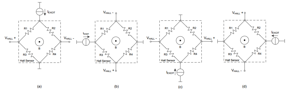
Figure 5. Current spinning technique used in the DRV411. Image courtesy of Texas Instruments
Another example is the ACS720 [PDF download link] from Allegro that is designed for open-loop current sensing applications. The ACS720 uses on-chip temperature compensation algorithms to optimize the accuracy over temperature.
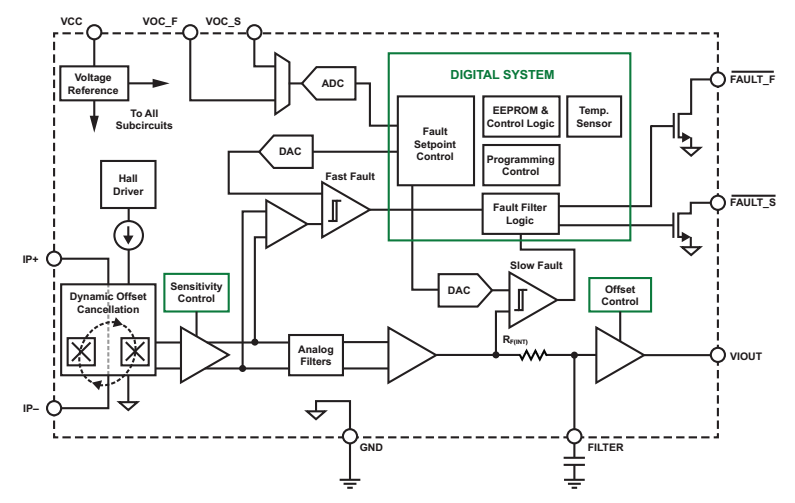
Figure 6. The block diagram of the ACS720. Image courtesy of Allegro Microsystems [PDF download link]
To see a complete list of my articles, please visit this page.
Related Content


Interesting article. Thanks for the effort. I just wish AAC made it available as a PDF so I could read it offline….had to make my own. I’ve seen current spinning before, applied to thermistors to avoid biases over time, but this was the first time I’ve seen it for current measurement.
Yes, PDF would be nice. Get mostly cut pictures and diagrams in my prints.