Facebook
 Google
 GitHub
 Linkedin
Thermocouple Cold Junction Compensation Using Analog Temperature Sensors
Learn how analog circuits can be used to implement cold junction compensation using examples from Analog Devices and Texas Instrument's TMP35 and LM335 temperature sensors, respectively.
Thermocouple look-up tables and mathematical models use a reference junction at 0 °C to specify the thermocouple output voltage. In practice, however, the cold junction is not usually at 0 °C, and signal conditioning electronics are required to correctly interpret the output voltage. This is known as cold junction compensation (CJC) in the context of thermocouples.
In this article, we’ll see how analog circuits can be used to implement cold junction compensation.
Cold Junction Compensation in an Analog Circuit
The basic idea of analog cold junction compensation is illustrated in Figure 1.
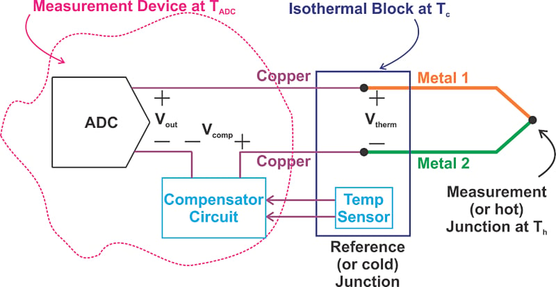
Figure 1. Overview diagram of analog cold junction compensation.
In Figure 1, we are assuming that the hot junction, cold junction, and the measurement system are respectively at Th, Tc, and TADC. The cold junction temperature (Tc) is measured by a temperature sensor (often a semiconductor sensor, sometimes a thermistor) and delivered to the “compensator circuit” to produce the appropriate compensating voltage term Vcomp. This voltage is added to the thermocouple output Vtherm; thus, the voltage measured by the ADC is:
$$V_{out}=V_{therm}+V_{comp}$$
From our previous article on cold junction compensation, we know that Vcomp is equal to the voltage produced by the thermocouple when its hot junction is at Tc, and its cold junction is at 0 °C. This voltage can be determined from the thermocouple reference table or mathematical model. Implementing a look-up table or a mathematical equation can be extremely challenging with analog circuits. Therefore, with an analog design, Vcomp can be only an approximate value of the actual thermocouple output.
Analog CJC circuits normally use a linear approximation to produce a compensating voltage close to the actual thermocouple output. This output is possible because the cold junction temperature typically changes in a relatively narrow range around the room temperature, which means that a linear approximation can produce relatively accurate values. In the next couple of sections, we’ll take a look at some example analog CJC diagrams.
Cold Junction Compensation Example 1—TMP35 Temperature Sensor
An example implementation of analog cold junction compensation is shown in Figure 2.
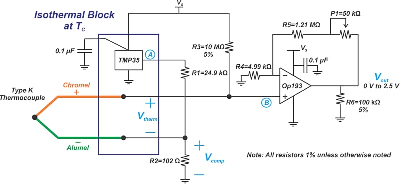
Figure 2. An example implementation of an analog cold junction compensation. Image [recreated] used courtesy of Analog Devices
In this case, the TMP35, a low voltage temperature sensor from Analog Devices, is used to measure the cold junction of a type K thermocouple. The non-inverting input of the op-amp measures the thermocouple output voltage, Vtherm, plus the voltage produced by the TMP35 divided down by the resistors R1 and R2 (Vcomp). Translated into mathematical language, the voltage at the non-inverting input, VB, is given by:
$$V_{B}=V_{therm}+V_{comp}$$
From the cold junction compensation theory, we know that Vcomp should be equal to the voltage that the 0 °C referenced thermocouple outputs when placed at a temperature of Tc where Tc is typically in a narrow range around the room temperature. Table 1 shows the output voltage of a Type K thermocouple over the temperature range from 0 °C to 50 °C.
Table 1. Data used courtesy of REOTEMP.
| °C | 0 | 1 | 2 | 3 | 4 | 5 | 6 | 7 | 8 | 9 | 10 |
| Thermoelectric Voltage in mV | |||||||||||
| 0 | 0.000 | 0.039 | 0.079 | 0.119 | 0.158 | 0.198 | 0.238 | 0.277 | 0.317 | 0.357 | 0.397 |
| 10 | 0.397 | 0.437 | 0.477 | 0.517 | 0.557 | 0.597 | 0.637 | 0.677 | 0.718 | 0.758 | 0.798 |
| 20 | 0.798 | 0.838 | 0.879 | 0.919 | 0.960 | 1.000 | 1.041 | 1.081 | 1.122 | 1.163 | 1.203 |
| 30 | 1.203 | 1.244 | 1.285 | 1.326 | 1.366 | 1.407 | 1.448 | 1.489 | 1.530 | 1.571 | 1.612 |
| 40 | 1.612 | 1.653 | 1.694 | 1.735 | 1.776 | 1.817 | 1.858 | 1.899 | 1.941 | 1.982 | 2.023 |
Figure 3 uses the above data (Table 1) to plot the type K thermocouple output against temperature.
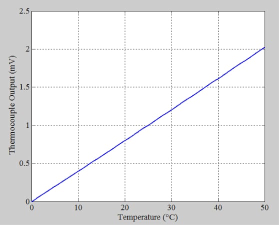
Figure 3. A plot showing the type K thermocouple output vs. temperature.
Over this restricted temperature range, the thermocouple appears to have a relatively linear response. For the compensator circuit to produce these values, Vcomp should have the same temperature coefficient as the employed thermocouple and go through an arbitrary point from the above characteristic curve. You can verify from the data in the table that the output of a type K thermocouple changes by about 41 μV/°C at room temperature (25 °C).
The voltage produced by the TMP35, node A in Figure 2, has a temperature coefficient of 10 mV/°C. To reduce this value to 41 μV/°C, we need a scaling factor of 41 μV/°C 10 mV/°C = 0.0041. This scaling factor is achieved through the resistive voltage divider formed by R1 and R2 as calculated below (Equation 1):
$$Attenuation\,Factor = \frac{R_{2}}{R_{1}+R_{2}}=\frac{0.102\,k\Omega}{24.9\,k\Omega+0.102\,l\Omega}\approx0.0041$$
Equation 1.
Now that Vcomp has the same temperature coefficient as the thermocouple, we need to ensure that it also goes through an arbitrary point from the characteristic curve of the thermocouple. The TMP35 produces an output of 250 mV at 25 °C. This value multiplied by 0.0041 (the attenuation factor) gives Vcomp = 1.025 mV which is close to the ideal output from the table (1 mV at 25 °C). Therefore, with the TMP35, we only need a resistive voltage divider to adjust the temperature coefficient of the semiconductor temperature sensor to that of the employed thermocouple, and an offset value is not required. To further clarify this discussion, let’s look at another example.
Cold Junction Compensation Example 2—LM335 Temperature Sensor
Another analog cold junction compensation circuit is shown in Figure 4.
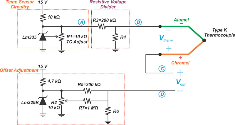
Figure 4. Another example implementation of cold junction compensation. Image [recreated] used courtesy of TI
To better understand this circuit, let’s first ignore the “offset adjustment” part of Figure 4 and find the voltage at node C. In this example, the LM335 is used to sense the cold junction temperature. The pot connected across the LM335 enables calibrating the temperature coefficient of the sensor output at the nominal value of 10 mV/°C. The output of the LM335 is proportional to the absolute temperature with the extrapolated output of the sensor going to zero volts at 0 K (−273.15 °C).
The error at the output of this sensor is only a slope error. As a result, the sensor calibration can be achieved by a single point calibration at an arbitrary temperature through the pot across the sensor. For example, to calibrate the TC of the sensor at 10 mV/°C, we can adjust the pot to have an output voltage of VA = 2.982 V at 25 °C as calculated below:
$$V_{A}\,@26°C=10mV/°C\times(25+273.15)\simeq2.982\,V$$
Similar to our previous example, the resistive voltage divider created by R3 and R4 divides down the 10 mV/°C temperature coefficient of the semiconductor sensor to that of the employed thermocouple. For example, with a type K thermocouple (41 μV/°C), we need a scaling factor of 41 μV/°C 10 mV/°C = 0.0041. Therefore, we should have:
$$\frac{R_{4}}{R_{4}+R_{3}}=0.0041$$
Assuming R3 = 200 kΩ, we obtain R4 = 823 Ω. This ensures that VB has a temperature coefficient of 41 μV/°C. The voltage at node C is given by Equation 2:
$$V_{C}=V_{therm}+V_{B}$$
Equation 2.
To achieve cold junction compensation, VB should have the same temperature coefficient as the employed thermocouple and go through an arbitrary point from the thermocouple output curve. At 25 °C, VA = 2.982 V and hence, VB=2.9820.0041 = 12.22 mV. From Table 1, the ideal output is 1 mV at 25 °C. Therefore, we need to subtract a DC value of 11.22 mV from Equation 2 to produce the appropriate compensating voltage. This is achieved through the “offset adjustment” part in Figure 4.
The LM329 is a precision temperature compensated 6.9 V voltage reference. If we ignore R7, the resistors R5 and R6 form a voltage divider. This voltage divider should attenuate 6.9 V to 11.22 mV at node D. Therefore, we have:
$$\frac{R_{6}}{R_{6}+R_{5}}=\frac{11.22mV}{6.9V}=0.0016$$
Assuming R5 = 200 kΩ, we obtain R6 = 320 Ω. Therefore, the overall output of the circuit is given by:
$$V_{out}=V_{C}-V_{D}=V_{therm}+V_{B}-V_{D}$$
Where VB-VD is the overall compensating voltage and produces the output voltage versus the temperature curve of a Type K thermocouple. R7 and R2 in Figure 4 allow us to fine-tune the DC voltage of node D and eliminate any constant error from resistor values, etc. In this article, we explained the basics of analog cold junction compensation circuits.
For additional information about the circuits in Figures 2 and 4, please refer to the “Linear Circuit Design Handbook” and “IC Temp Sensor Provides Thermocouple Cold-Junction Compensation” from Analog Devices and Texas Instruments, respectively.
To see a complete list of my articles, please visit this page.
Related Content