How to Build a Variational Autoencoder with TensorFlow

Over the years, we've seen many fields and industries leverage the power of artificial intelligence (AI) to push the boundaries of research. Data compression and reconstruction is no exception, where the application of artificial intelligence can be used to build more robust systems.

In this article, we are going to look at a very popular use-case of AI to compress data and reconstruct the compressed data with an autoencoder.

 

Autoencoder Applications

Autoencoders have gained the attention of many folks in machine learning, a fact made evident through the improvement of autoencoders and the invention of several variants. They have yielded some promising (if not state-of-the-art) results in several fields such as neural machine translation, drug discovery, image denoising, and several others.

 

Parts of the Autoencoder

Autoencoders, like most neural networks, learn by propagating gradients backwards to optimize a set of weights—but the most striking difference between the architecture of autoencoders and that of most neural networks is a bottleneck. This bottleneck is a means of compressing our data into a representation of lower dimensions. Two other important parts of an autoencoder are the encoder and decoder. 

Fusing these three components together forms a "vanilla" autoencoder, although more sophisticated ones may have some additional components.

Let’s take a look at these components independently.

 

Encoder

This is the first stage of data compression and reconstruction and it actually takes care of the data compression stage. The encoder is a feed-forward neural network which takes in data features (such as pixels in the case of image compression) and outputs a latent vector with a size that's less than the size of the data features. 

 

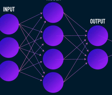
Image used courtesy of James Loy

 

To make reconstruction of the data robust, the encoder optimizes its weights during training to squeeze the most important features of the input data representation into the small-sized latent vector. This ensures that the decoder has enough information about the input data to reconstruct the data with minimal loss.

 

Latent Vector (Bottleneck)

The bottleneck or latent vector component of the autoencoder is the most crucial part—and it gets more crucial when we need to select its size.

The output of the encoder is what gives us the latent vector and is supposed to hold the most important feature representations of our input data. It also serves as input to the decoder part and propagates the useful representation to the decoder for reconstruction.

Choosing a smaller size for the latent vector means we get a representation of the input data features with less information about the input data. Choosing a much larger latent vector size sort of downplays the whole idea of compression with autoencoders and also increases computational cost.

 

Decoder

This stages concludes our data compression and reconstruction process. Just like the encoder, this component is also a feed-forward neural network, but it looks a little structurally different from the encoder. This difference comes from the fact that the decoder takes as input a latent vector of smaller size than that of the output from the decoder.

The function of the decoder is to generate an output from the latent vector that is very close to the input.

 

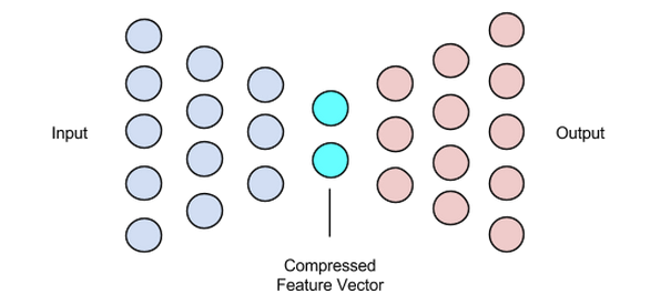
Image used courtesy of Chiman Kwan

 

Training Autoencoders

Usually, in training autoencoders, we build these components together instead of building them independently. We train them end-to-end with an optimization algorithm such as gradient descent or the ADAM optimizer.

 

Loss Functions

One portion of the autoencoder training procedure that's worth discussing is the loss function. Data reconstruction is a generation task and, unlike other machine learning tasks where our objective is to maximize the probability of predicting the correct class, we drive our network to produce an output close to the input.

We can achieve this objective with several loss functions such as l1, l2, mean squared error, and a couple of others. What these loss functions have in common is that they measure the difference (i.e., how far or identical) between input and output, making any of them a suitable choice.

 

Autoencoder Networks

All this while, we have been using a multi-layer perceptron to design both our encoder and decoder—but it turns out that we can use more specialized frameworks such as convolutional neural networks (CNNs) to capture more spatial information about our input data in the case of image data compression.

Surprisingly, research has shown that recurrent networks used as autoencoders for text data work very well, but we are not going to go into that in the scope of this article. The concept of an encoder-latent vector-decoder used in the multi-layer perceptron still holds for convolutional autoencoders. The only difference is that we design the decoder and encoder with convolutional layers.

All these autoencoder networks would work pretty well for the compression task, but there is one problem.

The networks we’ve discussed have zero creativity. What I mean by zero creativity is that they can only generate outputs they’ve seen or been trained with.

We can induce some level of creativity by tweaking our architecture design a bit. The outcome is known as a variational autoencoder.

 

Image used courtesy of Dawid Kopczyk

 

Variational Autoencoder

The variational autoencoder introduces two major design changes: 

• Instead of translating the input into a latent encoding, we output two parameter vectors: mean and variance.
• An additional loss term called the KL divergence loss is added to the initial loss function.

The idea behind the variational autoencoder is that we want our decoder to reconstruct our data using latent vectors sampled from distributions parameterized by a mean vector and variance vector generated by the encoder. 

Sampling features from a distribution grants the decoder a controlled space to generate from. After training a variational autoencoder, whenever we perform a forward pass with input data, the encoder generates a mean and variance vector responsible for determining the distribution from which to sample the latent vector.

The mean vector determines where the encoding of an input data should be centered around and the variance determines the radial space or circle where we want to pick the encoding from in order to generate a realistic output. This means that, with every forward pass with the same input data, our variational autoencoder can generate different variants of the output centered around the mean vector and within the variance space.

For comparison, when looking at a standard autoencoder, when we try to generate an output that the network hasn’t been trained on, it generates unrealistic outputs due to discontinuity in the latent vector space that the encoder produces.

 

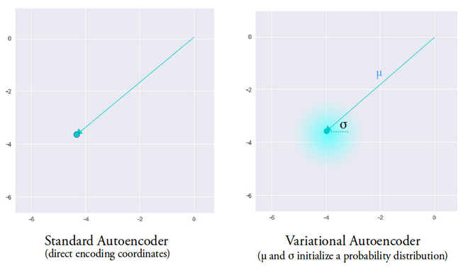
Image used courtesy of Irhum Shafkat

 

Now that we have an intuitive understanding of a variational autoencoder, let’s see how to build one in TensorFlow.

 

TensorFlow Code for a Variational Autoencoder

We’ll start our example by getting our dataset ready. For simplicity's sake, we’ll be using the MNIST dataset.

 

(train_images, _), (test_images, _) = tf.keras.datasets.mnist.load_data()

train_images = train_images.reshape(train_images.shape[0], 28, 28, 1).astype('float32')

test_images = test_images.reshape(test_images.shape[0], 28, 28, 1).astype('float32')

 

# Normalizing the images to the range of [0., 1.]

train_images /= 255.

test_images /= 255.

 

# Binarization

train_images[train_images >= .5] = 1.

train_images[train_images < .5] = 0.

test_images[test_images >= .5] = 1.

test_images[test_images < .5] = 0.

TRAIN_BUF = 60000

BATCH_SIZE = 100

 

TEST_BUF = 10000

train_dataset = tf.data.Dataset.from_tensor_slices(train_images).shuffle(TRAIN_BUF).batch(BATCH_SIZE)

test_dataset = tf.data.Dataset.from_tensor_slices(test_images).shuffle(TEST_BUF).batch(BATCH_SIZE)

Obtain dataset and prepare it for the task.

 

class CVAE(tf.keras.Model):

  def __init__(self, latent_dim):

    super(CVAE, self).__init__()

    self.latent_dim = latent_dim

    self.inference_net = tf.keras.Sequential(

      [

          tf.keras.layers.InputLayer(input_shape=(28, 28, 1)),

          tf.keras.layers.Conv2D(

              filters=32, kernel_size=3, strides=(2, 2), activation='relu'),

          tf.keras.layers.Conv2D(

              filters=64, kernel_size=3, strides=(2, 2), activation='relu'),

          tf.keras.layers.Flatten(),

          # No activation

          tf.keras.layers.Dense(latent_dim + latent_dim),

      ]

    )

 

    self.generative_net = tf.keras.Sequential(

        [

          tf.keras.layers.InputLayer(input_shape=(latent_dim,)),

          tf.keras.layers.Dense(units=7*7*32, activation=tf.nn.relu),

          tf.keras.layers.Reshape(target_shape=(7, 7, 32)),

          tf.keras.layers.Conv2DTranspose(

              filters=64,

              kernel_size=3,

              strides=(2, 2),

              padding="SAME",

              activation='relu'),

          tf.keras.layers.Conv2DTranspose(

              filters=32,

              kernel_size=3,

              strides=(2, 2),

              padding="SAME",

              activation='relu'),

          # No activation

          tf.keras.layers.Conv2DTranspose(

              filters=1, kernel_size=3, strides=(1, 1), padding="SAME"),

        ]

    )

 

  @tf.function

  def sample(self, eps=None):

    if eps is None:

      eps = tf.random.normal(shape=(100, self.latent_dim))

    return self.decode(eps, apply_sigmoid=True)

 

  def encode(self, x):

    mean, logvar = tf.split(self.inference_net(x), num_or_size_splits=2, axis=1)

    return mean, logvar

 

  def reparameterize(self, mean, logvar):

    eps = tf.random.normal(shape=mean.shape)

    return eps * tf.exp(logvar * .5) + mean

 

  def decode(self, z, apply_sigmoid=False):

    logits = self.generative_net(z)

    if apply_sigmoid:

      probs = tf.sigmoid(logits)

      return probs

 

    return logits

 

The two code snippets prepare our dataset and build our variational autoencoder model. In the model code snippet, there are a couple of helper functions to perform encoding, sampling, and decoding.

 

Reparameterization for Computing Gradients

There is a reparameterize function that we haven’t discussed but solves a very crucial problem in our variational autoencoder network. Recall that during the decoding stage, we sample the latent vector encoding from a distribution controlled by the mean and variance vector generated by the encoder. This generates no issue when forward propagating data through our network but causes a big problem when back-propagating gradients from the decoder to the encoder since the sampling operation is non-differentiable.

In simple terms, we can’t compute gradients from a sampling operation.

A nice workaround for this problem is to apply the reparameterization trick. This works by first generating a standard Gaussian distribution of mean 0 and variance 1 and then performing a differentiable addition and multiplication operation on this distribution with the mean and variance generated by the encoder.

Notice that we transform the variance into logarithm space in the code. This is to ensure numerical stability. The additional loss term, the Kullback-Leibler divergence loss, is introduced to ensure that the distributions we generate are as close to a standard Gaussian distribution with mean 0 and variance 1 as possible.

Driving the means of the distributions to zero ensures that the distributions we generate are very close to each other to prevent discontinuities between distributions. A variance close to 1 means we have a more moderate (i.e., not very large and not very small) space to generate encodings from.

 

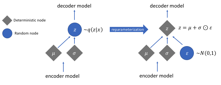
Image used courtesy of Jeremy Jordan

 

After performing the reparameterization trick, the distribution obtained by multiplying the variance vector with a standard Gaussian distribution and adding the result to the mean vector is very similar to distribution immediately controlled by the mean and variance vectors.

 

Simple Steps to Building a Variational Autoencoder

Let’s wrap up this tutorial by summarizing the steps in building a variational autoencoder:

1. Build the encoder and decoder networks.
2. Apply a reparameterizing trick between encoder and decoder to allow back-propagation.
3. Train both networks end-to-end.

The full code used above can be found on the official TensorFlow website.

 

Featured image modified from Chiman Kwan