Advanced Machine Learning with the Multilayer Perceptron

If you're interested in learning about neural networks, you've come to the right place. In this series, AAC's Director of Engineering will guide you through neural network terminology, example neural networks, and overarching theory.

Catch up on the series below:

1. How to Perform Classification Using a Neural Network: What Is the Perceptron?
2. How to Use a Simple Perceptron Neural Network Example to Classify Data
3. How to Train a Basic Perceptron Neural Network
4. Understanding Simple Neural Network Training
5. An Introduction to Training Theory for Neural Networks
6. Understanding Learning Rate in Neural Networks
7. Advanced Machine Learning with the Multilayer Perceptron
8. The Sigmoid Activation Function: Activation in Multilayer Perceptron Neural Networks
9. How to Train a Multilayer Perceptron Neural Network
10. Understanding Training Formulas and Backpropagation for Multilayer Perceptrons
11. Neural Network Architecture for a Python Implementation
12. How to Create a Multilayer Perceptron Neural Network in Python
13. Signal Processing Using Neural Networks: Validation in Neural Network Design
14. Training Datasets for Neural Networks: How to Train and Validate a Python Neural Network

 

---

 

Thus far we have focused on the single-layer Perceptron, which consists of an input layer and an output layer. As you might recall, we use the term “single-layer” because this configuration includes only one layer of computationally active nodes—i.e., nodes that modify data by summing and then applying the activation function. The nodes in the input layer just distribute data.

The single-layer Perceptron is conceptually simple, and the training procedure is pleasantly straightforward. Unfortunately, it doesn’t offer the functionality that we need for complex, real-life applications. I have the impression that a standard way to explain the fundamental limitation of the single-layer Perceptron is by using Boolean operations as illustrative examples, and that’s the approach that I’ll adopt in this article.

 

A Neural-Network Logic Gate

There’s something humorous about the idea that we would use an exceedingly sophisticated microprocessor to implement a neural network that accomplishes the same thing as a circuit consisting of a handful of transistors. At the same time, though, thinking about the issue in this way emphasizes the inadequacy of the single-layer Perceptron as a tool for general classification and function approximation—if our Perceptron can’t replicate the behavior of a single logic gate, we know that we need to find a better Perceptron.

Let’s go back to the system configuration that was presented in the first article of this series.

 

 

The general shape of this Perceptron reminds me of a logic gate, and indeed, that’s what it will soon be. Let’s say that we train this network with samples consisting of zeros and ones for the elements of the input vector and an output value that equals one only if both inputs equal one. The result will be a neural network that classifies an input vector in a way that is analogous to the electrical behavior of an AND gate.

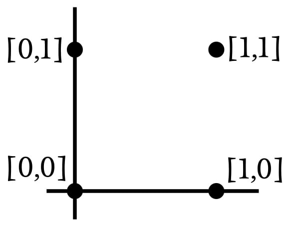
The dimensionality of this network’s input is 2, so we can easily plot the input samples in a two-dimensional graph. Let’s say that input0 corresponds to the horizontal axis and input1 corresponds to the vertical axis. The four possible input combinations will be arranged as follows:

 

   

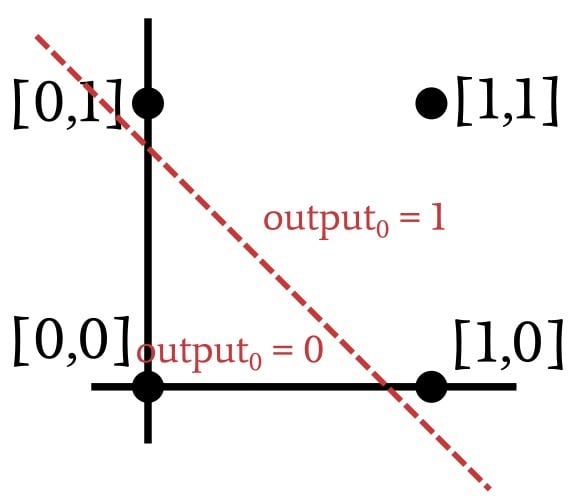
Since we’re replicating the AND operation, the network needs to modify its weights such that the output is one for input vector [1,1] and zero for the other three input vectors. Based on this information, let’s divide the input space into sections corresponding to the desired output classifications:

 

  

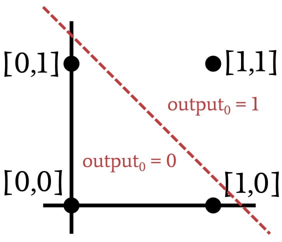
Linearly Separable Data

As demonstrated by the previous plot, when we’re implementing the AND operation, the plotted input vectors can be classified by drawing a straight line. Everything on one side of the line receives an output value of one, and everything on the other side receives an output value of zero. Thus, in the case of an AND operation, the data that are presented to the network are linearly separable. This would also be the case with an OR operation:

 

 

It turns out that a single-layer Perceptron can solve a problem only if the data are linearly separable. This is true regardless of the dimensionality of the input samples. The two-dimensional case is easy to visualize because we can plot the points and separate them with a line. To generalize the concept of linear separability, we have to use the word “hyperplane” instead of “line.” A hyperplane is a geometric feature that can separate data in n-dimensional space. In a two-dimensional environment, a hyperplane is a one-dimensional feature (i.e., a line). In a three-dimensional environment, a hyperplane is an ordinary two-dimensional plane. In an n-dimensional environment, a hyperplane has (n-1) dimensions.

 

Solving Problems That Are Not Linearly Separable

During the training procedure, a single-layer Perceptron is using the training samples to figure out where the classification hyperplane should be. After it finds the hyperplane that reliably separates the data into the correct classification categories, it is ready for action. However, the Perceptron won’t find that hyperplane if it doesn’t exist. Let’s look at an example of an input-to-output relationship that is not linearly separable:

 

 

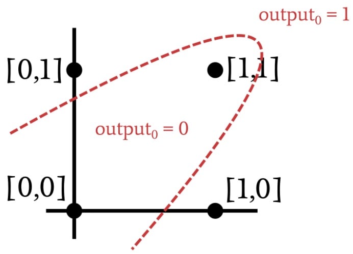
Do you recognize that relationship? Take another look and you’ll see that it’s nothing more than the XOR operation. You can’t separate XOR data with a straight line. Thus, a single-layer Perceptron cannot implement the functionality provided by an XOR gate, and if it can’t perform the XOR operation, we can safely assume that numerous other (far more interesting) applications will be beyond the reach of the problem-solving capabilities of a single-layer Perceptron.

Fortunately, we can vastly increase the problem-solving power of a neural network simply by adding one additional layer of nodes. This turns the single-layer Perceptron into a multi-layer Perceptron (MLP). As mentioned in a previous article, this layer is called “hidden” because it has no direct interface with the outside world. I suppose you could think of an MLP as the proverbial “black box” that accepts input data, performs mysterious mathematical operations, and produces output data. The hidden layer is inside that black box. You can’t see it, but it’s there.

 

Conclusion

Adding a hidden layer to the Perceptron is a fairly simple way to greatly improve the overall system, but we can’t expect to get all that improvement for nothing. The first disadvantage that comes to mind is that training becomes more complicated, and this is the issue that we’ll explore in the next article.