 Facebook
 Google
 GitHub
 Linkedin
Training Datasets for Neural Networks: How to Train and Validate a Python Neural Network
In this article, we’ll use Excel-generated samples to train a multilayer Perceptron, and then we’ll see how the network performs with validation samples.
If you're looking to develop a Python neural network, you're in the right place. Before delving into this article's discussion of how to use Excel to develop training data for your network, consider checking out the rest of the series below for background info:
- How to Perform Classification Using a Neural Network: What Is the Perceptron?
- How to Use a Simple Perceptron Neural Network Example to Classify Data
- How to Train a Basic Perceptron Neural Network
- Understanding Simple Neural Network Training
- An Introduction to Training Theory for Neural Networks
- Understanding Learning Rate in Neural Networks
- Advanced Machine Learning with the Multilayer Perceptron
- The Sigmoid Activation Function: Activation in Multilayer Perceptron Neural Networks
- How to Train a Multilayer Perceptron Neural Network
- Understanding Training Formulas and Backpropagation for Multilayer Perceptrons
- Neural Network Architecture for a Python Implementation
- How to Create a Multilayer Perceptron Neural Network in Python
- Signal Processing Using Neural Networks: Validation in Neural Network Design
- Training Datasets for Neural Networks: How to Train and Validate a Python Neural Network
What Is Training Data?
In a real-life scenario, training samples consist of measured data of some kind combined with the “solutions” that will help the neural network to generalize all this information into a consistent input–output relationship.
For example, let’s say that you want your neural network to predict the eating quality of a tomato based on color, shape, and density. You have no idea how exactly the color, shape, and density are correlated with overall deliciousness, but you can measure color, shape, and density, and you do have taste buds. Thus, all you need to do is gather thousands upon thousands of tomatoes, record their relevant physical characteristics, taste each one (the best part), and then put all this information into a table.
Each row is what I call one training sample, and there are four columns: three of these (color, shape, and density) are input columns, and the fourth is the target output.
During training, the neural network will find the relationship (if a coherent relationship exists) between the three input values and the output value.
Quantifying Training Data
Keep in mind that everything has to be processed in numerical form. You can’t use the string “plum-shaped” as an input to your neural network, and “mouthwatering” won’t work as an output value. You need to quantify your measurements and your classifications.
For shape, you might assign each tomato a value from –1 to +1, where –1 represents perfectly spherical and +1 represents extremely elongated. For eating quality, you could rate each tomato on a five-point scale ranging from “inedible” to “delectable” and then use one-hot encoding to map the ratings to a five-element output vector.
The following diagram shows you how this type of encoding is employed for neural-network output classification.
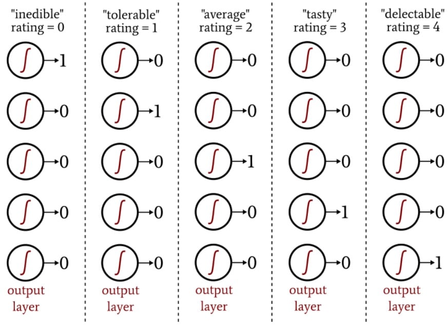
The one-hot output scheme allows us to quantify non-binary classifications in a way that is compatible with logistic-sigmoid activation. The output of the logistic function is essentially binary because the curve’s transition region is narrow compared to the infinite range of input values for which the output value is very close to the minimum or maximum:
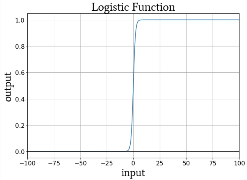
Thus, we don’t want to configure this network with a single output node and then supply training samples that have output values of 0, 1, 2, 3, or 4 (that would be 0, 0.2, 0.4, 0.6, or 0.8 if you want to stay in the 0-to-1 range); the output node’s logistic activation function would strongly favor the minimum and maximum ratings.
The neural network just doesn’t understand how preposterous it would be to conclude that all tomatoes are either inedible or delectable.
Creating a Training Data Set
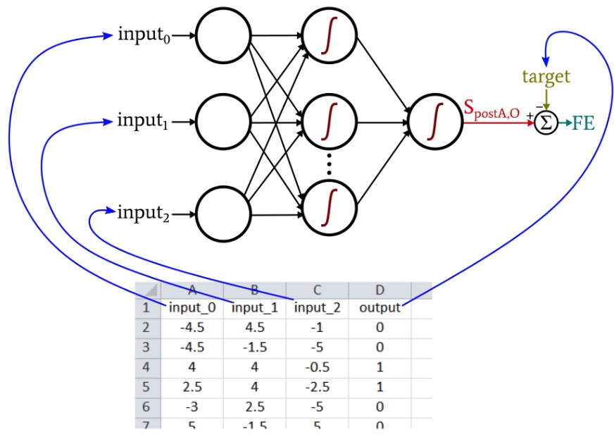
The Python neural network that we discussed in Part 12 imports training samples from an Excel file. The training data that I will use for this example are organized as follows:
Our current Perceptron code is limited to one output node, so all we can do is perform a true/false type of classification. The input values are random numbers between –5 and +5, generated using this Excel formula:
=RANDBETWEEN(-10, 10)/2
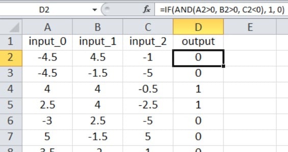
As shown in the screenshot, the output is calculated as follows:
=IF(AND(A2>0, B2>0, C2<0), 1, 0)
Thus, the output is true only if input_0 is greater than zero, input_1 is greater than zero, and input_2 is less than zero. Otherwise, it’s false.
This is the mathematical input–output relationship that the Perceptron needs to extract from the training data. You can generate as many samples as you like. For a simple problem like this one, you can achieve very high classification accuracy with 5000 samples and one epoch.
Training the Network
You’ll need to set your input dimensionality to three (I_dim = 3, if you’re using my variable names). I configured the network to have four hidden nodes (H_dim = 4), and I chose a learning rate of 0.1 (LR = 0.1).
Find the training_data = pandas.read_excel(...) statement and insert the name of your spreadsheet. (If you don’t have access to Excel, the Pandas library can also read ODS files.) Then just click the Run button. Training with 5000 samples takes only a few seconds on my 2.5 GHz Windows laptop.
If you’re using the complete “MLP_v1.py” program that I included in Part 12, validation (see the next section) begins immediately after training is complete, so you’ll need to have your validation data ready before you train the network.
Validating the Network
To validate the performance of the network, I create a second spreadsheet and generate input and output values using the exact same formulas, and then I import this validation data in the same way that I import training data:
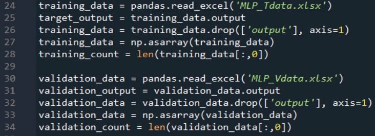
The next code excerpt shows you how you can perform basic validation:
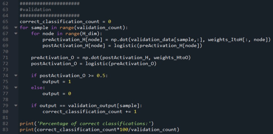
I use the standard feedforward procedure to calculate the output node’s postactivation signal, and then I use an if/else statement to apply a threshold that converts the postactivation value into a true/false classification value.
Classification accuracy is computed by comparing the classification value to the target value for the current validation sample, counting the number of correct classifications, and dividing by the number of validation samples.
Remember that if you have the np.random.seed(1) instruction commented out, the weights will initialize to different random values each time you run the program, and consequently, the classification accuracy will change from one run to the next. I performed 15 separate runs with the parameters specified above, 5000 training samples, and 1000 validation samples.
The lowest classification accuracy was 88.5%, the highest was 98.1%, and the average was 94.4%.
Conclusion
We’ve covered some important theoretical information related to neural-network training data, and we did an initial training and validation experiment with our Python-language multilayer Perceptron. I hope that you’re enjoying AAC’s series on neural networks—we’ve made a lot of progress since the first article, and there’s still much more that we need to discuss!


This all was obsolesced in 2017.
Hi, may I have your email address?
Hello.
The question is what to do if there is more than one output node?
How to change the program so that the learning algorithm works correctly.
Sample data in the screenshot
I will be very grateful for the answer!