Facebook
 Google
 GitHub
 Linkedin
How to Train a Multilayer Perceptron Neural Network
We can greatly enhance the performance of a Perceptron by adding a layer of hidden nodes, but those hidden nodes also make training a bit more complicated.
So far in the AAC series on neural networks, you've learned about data classification using neural networks, especially of the Perceptron variety.
Catch up on the series below or dive into this new entry which will explain the basics of the multilayer Perceptron (MLP) neural network.
- How to Perform Classification Using a Neural Network: What Is the Perceptron?
- How to Use a Simple Perceptron Neural Network Example to Classify Data
- How to Train a Basic Perceptron Neural Network
- Understanding Simple Neural Network Training
- An Introduction to Training Theory for Neural Networks
- Understanding Learning Rate in Neural Networks
- Advanced Machine Learning with the Multilayer Perceptron
- The Sigmoid Activation Function: Activation in Multilayer Perceptron Neural Networks
- How to Train a Multilayer Perceptron Neural Network
- Understanding Training Formulas and Backpropagation for Multilayer Perceptrons
- Neural Network Architecture for a Python Implementation
- How to Create a Multilayer Perceptron Neural Network in Python
- Signal Processing Using Neural Networks: Validation in Neural Network Design
- Training Datasets for Neural Networks: How to Train and Validate a Python Neural Network
What Is a Multilayer Perceptron Neural Network?
The previous article demonstrated that a single-layer Perceptron simply cannot produce the sort of performance that we expect from a modern neural-network architecture. A system that is limited to linearly separable functions will not be able to approximate the complex input–output relationships that occur in real-life signal-processing scenarios. The solution is a multilayer Perceptron (MLP), such as this one:
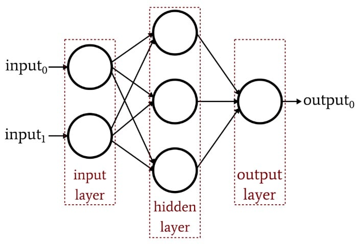
By adding that hidden layer, we turn the network into a “universal approximator” that can achieve extremely sophisticated classification. But we always have to remember that the value of a neural network is completely dependent on the quality of its training. Without abundant, diverse training data and an effective training procedure, the network will never “learn” how to classify input samples.
Why Does the Hidden Layer Complicate Training?
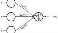
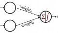
Let’s look at the learning rule that we used to train a single-layer Perceptron in a previous article:
\[w_{new} = w+(\alpha\times(output_{expected}-output_{calculated})\times input)\]
Notice the implicit assumption in this equation: We update the weights based on the observed output, so for this to work, the weights in the single-layer Perceptron must directly influence the output value. It’s like choosing the temperature of faucet water by turning the two knobs for hot and cold. The relationship between overall temperature and knob action is fairly straightforward, and even folks who don’t like math can find the desired water temperature by fiddling with the knobs for a little while.
But now imagine that the flow of water through the hot and cold pipes is related to knob position in a complex, highly nonlinear way. You steadily and slowly turn the knob for hot water, but the resulting flow rate is varying erratically. You try the knob for cold water and it does the same thing. Settling on the ideal water temperature under these conditions—especially since the “output” must be achieved through a combination of two confusing control relationships—would be much more difficult.
This is how I understand the dilemma of the hidden layer. The weights that connect the input nodes to the hidden nodes are conceptually analogous to those mechanically erratic knobs—because input-to-hidden weights don’t have a direct path to the output layer, the relationship between these weights and the network’s output is so complex that the simple learning rule shown above will not be effective.
A New Training Paradigm
Since the original Perceptron learning rule cannot be applied to multilayer networks, we need to rethink our training strategy. What we’re going to do is incorporate gradient descent and minimization of an error function.
One thing to keep in mind is that this training procedure is not specific to multilayer neural networks. Gradient descent comes from general optimization theory, and the training procedure that we employ for MLPs is also applicable to single-layer networks. However, as I understand it, MLP-style gradient descent is (at least theoretically) unnecessary for a single-layer Perceptron, because the simpler rule shown above will eventually get the job done.
Deriving the actual weight-update equations for an MLP involves some intimidating math that I won’t attempt to intelligently explain at this juncture. My objective for the rest of this article is to provide a conceptual introduction to two key aspects of MLP training—gradient descent and the error function—and then we’ll continue this discussion in the next article by incorporating a new activation function.
Gradient Descent
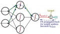
As the name implies, gradient descent is a means of descending toward the minimum of an error function based on slope. The diagram below conveys the way in which a gradient gives us information about how to modify weights—the slope of a point on the error function tells us which direction we need to go and how far away we are from the minimum.
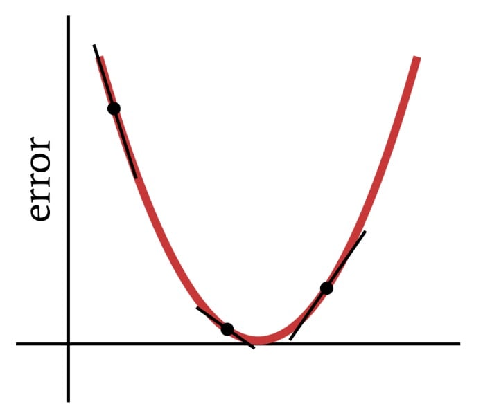
Thus, the derivative of the error function is an important element of the computations that we use to train a multilayer Perceptron. Actually, we’ll need partial derivatives here. When we implement gradient descent, we make each weight modification proportional to the slope of the error function with respect to the weight being modified.
The Error Function (AKA Loss Function)
A common method of quantifying a neural network’s error is to square the difference between the expected (or “target”) value and the calculated value for each output node, and then sum all these squared differences. You can call this “sum of squared difference” or “summed squared error” or maybe various other things, and you will also see the abbreviation LMS, which stands for least-mean-square, because the goal of training is to minimize the mean squared error. This error function (denoted by E) can be mathematically expressed as follows:
\[E=\frac{1}{2}\sum_k(t_k-o_k)^2\]
where k indicates the range of output nodes, t is the target output value, and o is the calculated output value.
Conclusion
We’ve laid the groundwork for successfully training a multilayer Perceptron, and we’ll continue exploring this interesting topic in the next article.
Related Content