Neural Network Architecture for a Python Implementation

Welcome to the All About Circuits neural network series of technical articles. In the series so far—linked below—we’ve covered quite a bit of theory surrounding neural networks.

1. How to Perform Classification Using a Neural Network: What Is the Perceptron?
2. How to Use a Simple Perceptron Neural Network Example to Classify Data
3. How to Train a Basic Perceptron Neural Network
4. Understanding Simple Neural Network Training
5. An Introduction to Training Theory for Neural Networks
6. Understanding Learning Rate in Neural Networks
7. Advanced Machine Learning with the Multilayer Perceptron
8. The Sigmoid Activation Function: Activation in Multilayer Perceptron Neural Networks
9. How to Train a Multilayer Perceptron Neural Network
10. Understanding Training Formulas and Backpropagation for Multilayer Perceptrons
11. Neural Network Architecture for a Python Implementation
12. How to Create a Multilayer Perceptron Neural Network in Python
13. Signal Processing Using Neural Networks: Validation in Neural Network Design
14. Training Datasets for Neural Networks: How to Train and Validate a Python Neural Network

Now we’re ready to start converting this theoretical knowledge into a functional Perceptron classification system.

First I want to introduce the general characteristics of the network that we will implement in a high-level programming language; I’m using Python, but the code will be written in a way that facilitates translation to other languages such as C. The next article provides the detailed walk-through of the Python code, and after that we’ll explore different ways of training, using, and evaluating this network.

 

The Python Neural Network Architecture

The software corresponds to the Perceptron depicted in the following diagram.

 

 

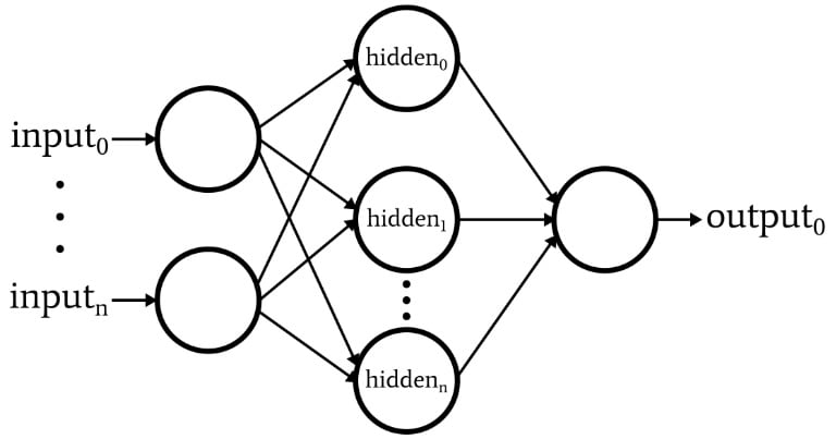
Here are the basic characteristics of the network:

• The number of input nodes is variable. This is essential if we want a network that has any significant degree of flexibility, because the input dimensionality must match the dimensionality of the samples that we want to classify.
• The code does not support multiple hidden layers. At this point there’s no need—one hidden layer is enough for extremely powerful classification.
• The number of nodes within the one hidden layer is variable. Finding the optimal number of hidden nodes involves some trial and error, though there are guidelines that can help us to choose a reasonable starting point. We’ll explore the issue of hidden-layer dimensionality in a future article.
• The number of output nodes is currently fixed at one. This limitation will make our initial program a bit simpler, and we can incorporate variable output dimensionality into an improved version.
• The activation function for both hidden and output nodes will be the standard logistic sigmoid relationship:

 

\[f(x)=\frac{1}{1+e^{-x}}\]

 

What Is a Bias Node? (AKA Bias Is Good If You’re a Perceptron)

While we’re discussing network architecture, I should point out that neural networks often incorporate something called a bias node (or you can call it just a “bias,” without “node”). The numerical value associated with a bias node is a constant chosen by the designer. For example:

 

 

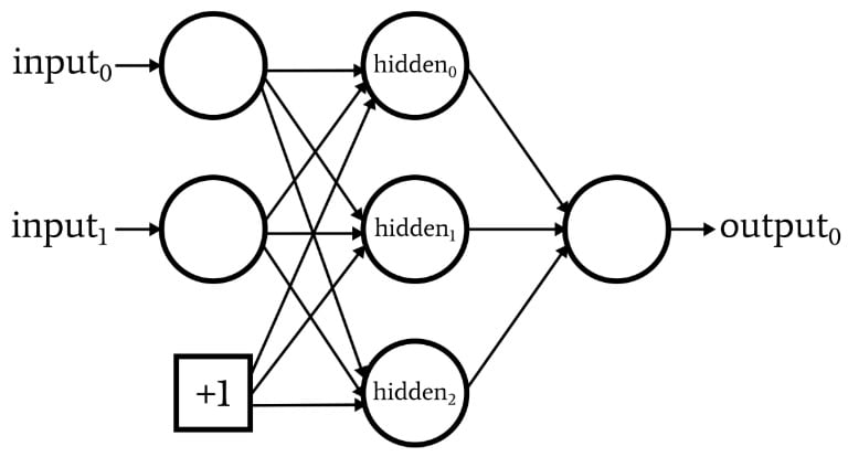
Bias nodes can be incorporated into the input layer or the hidden layer, or both. Their weights are like any other weights and are updated using the same backpropagation procedure.

The use of bias nodes is an important reason to write neural-network code that allows you to easily change the number of input nodes or hidden nodes—even if you are interested only in one specific classification task, variable input- and hidden-layer dimensionality ensures that you can conveniently experiment with the use of bias nodes.

In Part 10, I pointed out that a node’s preactivation signal is computed by performing a dot product—i.e., you multiply the corresponding elements of two arrays (or vectors, if you prefer) and then add up all the individual products. The first array holds the postactivation values from the preceding layer, and the second array holds the weights that connect the preceding layer to the current layer. Thus, if the preceding-layer postactivation array is denoted by x and the weight vector is denoted by w, a preactivation value is calculated as follows:

 

\[S_{preA} = w \cdot x = sum(w_1x_1 + w_2x_2 + \cdots + w_nx_n)\]

 

You might be wondering what on earth this has to do with bias nodes. Well, the bias (denoted by b) modifies this procedure as follows:

 

\[S_{preA} =( w \cdot x)+b = sum(w_1x_1 + w_2x_2 + \cdots + w_nx_n)+b\]

 

A bias shifts the signal that is processed by the activation function, and it can thereby make the network more flexible and robust. The use of the letter b to denote the bias value is reminiscent of the “y-intercept” in the standard equation for a straight line: y = mx + b. And this is no idle coincidence. The bias is indeed like a y-intercept, and you may also have noticed that the array of weights is equivalent to a slope:

 

\[S_{preA} =( w \cdot x)+b\]

\[y = mx + b\]

 

Weights, Bias, and Activation

If we think about the numerical values delivered to a node’s activation function during training, the weights increase or decrease the slope of the input data, and the bias shifts the input data vertically. But how does this affect the node’s output? Well, let’s assume that we’re using the standard logistic function for activation:

 

  

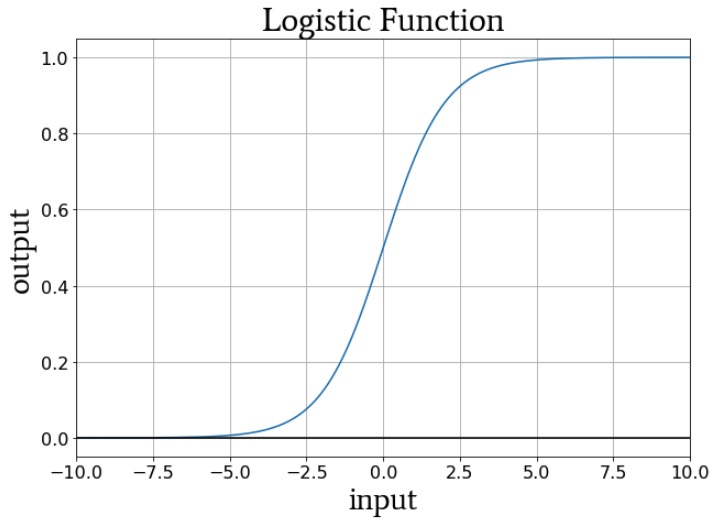
The transition from f_A(x) = 0 to f_A(x) = 1 is centered on an input value of x = 0. Thus, by using a bias to increase or decrease the preactivation signal, we can influence the occurrence of the transition and thereby shift the activation function to the left or the right. The weights, on the other hand, determine how “quickly” the input value passes through x = 0, and this influences the steepness of the transition in the activation function.

 

Conclusion

We’ve discussed bias nodes and the salient characteristics of the first neural network that we will implement in software. Now we’re ready to look at the actual code, and that’s exactly what we’ll do in the next article.