The Sigmoid Activation Function: Activation in Multilayer Perceptron Neural Networks

Welcome to the All About Circuits neural network series developed by Director of Engineering Robert Keim. You can catch up on the series using the guide below:

1. How to Perform Classification Using a Neural Network: What Is the Perceptron?
2. How to Use a Simple Perceptron Neural Network Example to Classify Data
3. How to Train a Basic Perceptron Neural Network
4. Understanding Simple Neural Network Training
5. An Introduction to Training Theory for Neural Networks
6. Understanding Learning Rate in Neural Networks
7. Advanced Machine Learning with the Multilayer Perceptron
8. The Sigmoid Activation Function: Activation in Multilayer Perceptron Neural Networks
9. How to Train a Multilayer Perceptron Neural Network
10. Understanding Training Formulas and Backpropagation for Multilayer Perceptrons
11. Neural Network Architecture for a Python Implementation
12. How to Create a Multilayer Perceptron Neural Network in Python
13. Signal Processing Using Neural Networks: Validation in Neural Network Design
14. Training Datasets for Neural Networks: How to Train and Validate a Python Neural Network

In this article, you'll learn about activation functions, including the limitations associated with unit-step activation functions and how the sigmoid activation function can make up for them in multilayer Perceptron neural networks.

Why Unit-step Activation Functions Aren't Suitable for Multilayer Perceptrons

Thus far in our series, we’ve been using the unit-step activation function:

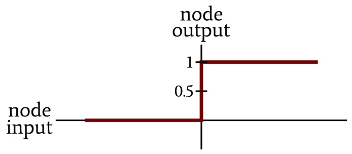
The network’s computational nodes summed all the weighted values delivered by the preceding layer and then converted these sums to one or zero according to the following expression:

\[f(x)=\begin{cases}0 & x < 0\\1 & x \geq 0\end{cases}\]

However, you may have noticed that in my network diagrams, the representation of the activation function is not a unit step. It’s more like a smoothed, not-quite-vertical version of the unit step:

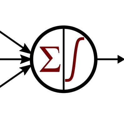
The smoothed version is more visually appealing, in my opinion, but that’s not the reason why I chose it. Or at least that’s not the only reason. It turns out that the unit step is not a good activation function for multilayer Perceptrons.

Let’s find out why.

Gradient Descent with Summed Squared Error

Summed squared error is our error function, and updating weights via gradient descent requires that we find the partial derivative of the error function with respect to the weight that we want to update. Performing this differentiation reveals that the error gradient with respect to a weight is given by an expression that includes the derivative of the activation function.

The unit step allows the calculations that occur within the node to be very simple (all you need is an if/else statement), but this benefit becomes meaningless in the context of gradient descent because the unit step is not differentiable—it’s not a continuous function, and the slope at the point where the output transitions from zero to one is infinity.

If we intend to train a neural network using gradient descent, we need a differentiable activation function. Since the unit step is consistent with the on/off behavior of biological neurons and theoretically effective (though limited) within systems consisting of artificial neurons, it makes sense to consider an activation function that is similar to the unit step but without the lack of differentiability. We need look no further than the logistic sigmoid function.

The Sigmoid Activation Function

The adjective “sigmoid” refers to something that is curved in two directions. There are various sigmoid functions, and we’re only interested in one. It’s called the logistic function, and the mathematical expression is fairly straightforward:

\[f(x)=\frac{L}{1+e^{-kx}}\] 

The constant L determines the curve’s maximum value, and the constant k influences the steepness of the transition. The plot below shows examples of the logistic function for different values of L, and the following plot shows curves for different values of k.

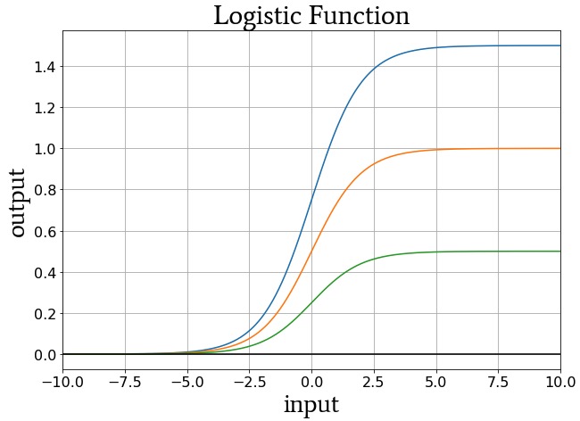
Logistic-function curves for L = 1.5 (blue), L = 1 (orange), and L = 0.5 (green).

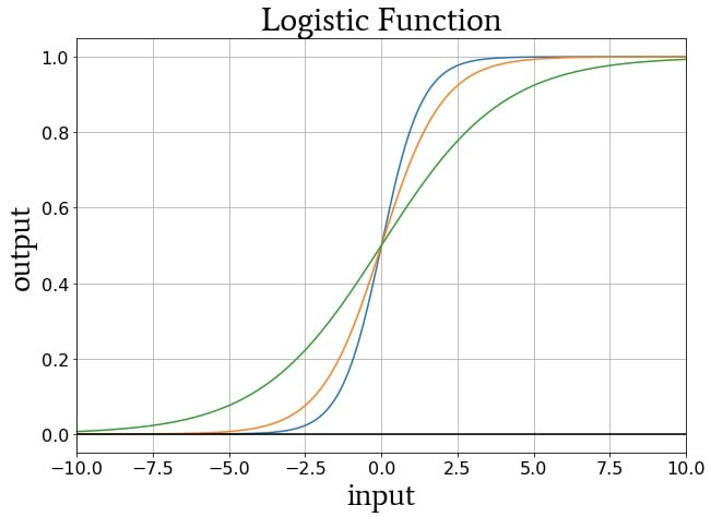
Logistic-function curves for k = 1.5 (blue), k = 1 (orange), and k = 0.5 (green).

The logistic function is not the only activation function used in MLPs, but it is very common and has multiple benefits:

• As mentioned above, logistic activation is an excellent improvement upon the unit step because the general behavior is equivalent, but the smoothness in the transition region ensures that the function is continuous and therefore differentiable.
• The computational burden certainly exceeds that of the unit step, but it still seems fairly reasonable to me—just one exponential operation, one addition, and one division.
• We can easily fine-tune the input–output relationship by adjusting the L and k parameters. However, I believe that neural networks typically use the standard logistic function, i.e., with L = 1 and k = 1.
• The shape of the logistic curve—high derivative near the middle of the output range and low derivative for outputs near the maximum and minimum values—might promote successful training. I can’t claim authoritative expertise on such matters, so I’ll quote directly from a book on parallel distributed processing made available by Stanford University: since weight modifications are proportional to the derivative of the activation function, weight changes will be larger for nodes that are “not yet committed to being either on or off,” and this may “[contribute] to the stability of the learning of the system.”

The Derivative of the Logistic Function

The standard logistic function, f(x), has the following first derivative:

\[f(x)=\frac{1}{1+e^{-x}} \ \ \Rightarrow \ \ f^\prime(x)=\frac{e^x}{(1+e^x)^2}\]

However, if you have already calculated the output of the logistic function for a given input value, you don’t need to use the expression for the derivative, because it turns out that the derivative of the logistic function is related to the original logistic function as follows:

\[f^\prime(x)=f(x)(1-f(x))\]

Conclusion

I hope that you now have a clear idea of what the logistic sigmoid function is and why we use it for activation in multilayer Perceptrons. The logistic function is undoubtedly effective, and I have successfully used it to design neural networks. However, it becomes less desirable as the number of hidden layers increases, because of something called the vanishing gradient problem. Maybe we’ll explore the vanishing gradient problem and other more-advanced issues in future articles.