An Introduction to Training Theory for Neural Networks

This article is part of AAC's series on neural networks. You can find the rest of the series below if you'd like to catch up before moving forward:

1. How to Perform Classification Using a Neural Network: What Is the Perceptron?
2. How to Use a Simple Perceptron Neural Network Example to Classify Data
3. How to Train a Basic Perceptron Neural Network
4. Understanding Simple Neural Network Training
5. An Introduction to Training Theory for Neural Networks
6. Understanding Learning Rate in Neural Networks
7. Advanced Machine Learning with the Multilayer Perceptron
8. The Sigmoid Activation Function: Activation in Multilayer Perceptron Neural Networks
9. How to Train a Multilayer Perceptron Neural Network
10. Understanding Training Formulas and Backpropagation for Multilayer Perceptrons
11. Neural Network Architecture for a Python Implementation
12. How to Create a Multilayer Perceptron Neural Network in Python
13. Signal Processing Using Neural Networks: Validation in Neural Network Design
14. Training Datasets for Neural Networks: How to Train and Validate a Python Neural Network

In this article, we'll go over the theory and practice of neural network training and address the concept of the error bowl. 

 

Training: Theory vs. Practice

At first glance, neural-network training seems fairly straightforward. When we’re working with a simple network (such as the single-layer Perceptron shown below), the math required for training is certainly not overwhelming, the network itself can be implemented in a relatively short program written in common languages such as C or Python, and the training process doesn’t require excessive amounts of computational time.

Also, the general concept is reminiscent of the settling action associated with negative feedback: we apply an input, produce an output, compare the produced output to the expected output, and feed that information back into the network in a way that allows the weights to gradually converge on values that are appropriate for the task at hand.

 

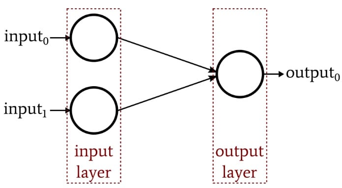
A single-layer Perceptron neural network.

 

However, as you probably already know or have already guessed, there is quite a bit of theory associated with the training of artificial neural networks—do a search for “neural network training” in Google Scholar and you’ll get a good sample of the research that has been conducted in this area. One title that caught my eye was “A simple lemma on greedy approximation in Hilbert space and convergence rates for projection pursuit regression and neural network training.” If you know what that means, you’re several steps ahead of me and should probably be writing your own articles rather than reading mine.

Fortunately, I won’t be quoting from any academic publications in this article. Our objective at this point is to understand one foundational concept, namely, error minimization.

 

Perceptron as Universal Approximator

A neural network can perform classification because it automatically finds and implements (via training) a mathematical relationship between input data and output values. In mathematical terminology, we use the word “function” to identify an input–output relationship, and we often express functions symbolically as f(x), e.g., f(x) = sin(x). Thus, x represents the input data, and f(x) is set equal to the procedure that we use when we want the function to operate on the input and produce an output.

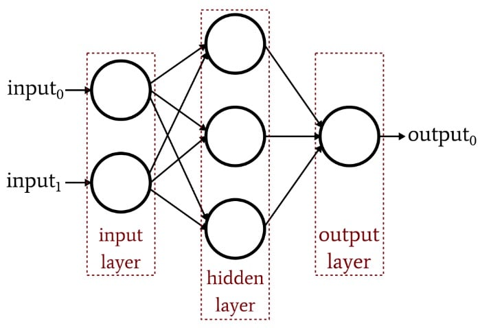
A Perceptron that includes an additional layer of nodes (i.e., more than just the input and output layer) is called a multilayer Perceptron, or MLP. These nodes constitute a hidden layer, because they aren’t directly “visible” from the input side or the output side. This architecture is shown in the diagram below and will be explored thoroughly in future articles.

 

 

A multilayer Perceptron is considered a universal approximator. There are various nuances associated with this concept, but the general idea is that the math performed by the network allows for immense flexibility in the overall function—I mean function as in f(x), i.e., the relationship between input and output—created by the network’s mathematical operations.

When the network first starts training, random values have been assigned to the weights, and consequently the network’s f(x)—we’ll call this f_NN(x)—is not at all consistent with the real relationship, f_REAL(x), between input and output. During training, the network generates beneficial adjustments in weight values by looking at error information fed back from the output, and f_NN(x) gradually becomes more and more consistent with f_REAL(x), kind of like a precise reflection that slowly appears as condensation evaporates from a mirror. (Note: In this case, the symbol x doesn’t represent one variable, as though the dimensionality of the network’s input layer is one. It represents input data in a generic way. For example, x could be a 50-element vector.)  

 

The Error Bowl

Let’s assume that we’re working with a neural network that has two weighted connections leading to a single output node. If we’re training, we know the correct output value, and consequently we can calculate the error produced by this output node. Furthermore, we can visualize the error using a three-dimensional plot: the two inputs correspond to the x-axis and the y-axis, and the error corresponds to the z-axis.

The fundamental idea here is that each combination of input weights and output error is like a point in three-dimensional space. As the weights are modified, the x and y components of the point change, and the z component will change as well if the weight modification produces a change in error. As the weights improve, the error decreases toward zero, and this is represented by the three-dimensional error bowl shown below.

 

      

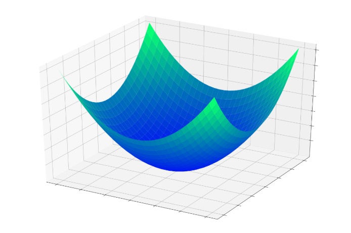
The training procedure is essentially a quest for the bottom of that bowl, where z = 0, because if z = 0, the output produced by the node is equal to the expected output. As the weights are gradually adjusted during training, the point defined by the two weights and the error is moving along the surface of that bowl, hopefully heading downward. 

This visual analogy brings us back to the concept of function approximation: descent toward the minimum error occurs as the weights are changing, and the changes in the weights are also what makes f_NN(x) gradually resemble f_REAL(x). To summarize, then, training forces the network to modify its weights in a way that results in minimization of the error function and that causes the mathematical operations of the overall network to approximate the mathematical relationship between input and output.

 

Conclusion

I hope that this article has given you a more thorough understanding of neural-network training. In the next article, we’ll continue this topic with a discussion of learning rate.