 Facebook
 Google
 GitHub
 Linkedin
Integrator Limitations: The Op-Amp’s Output Impedance
In this second part of a series of articles, we investigate the role of the output impedance of a real-life op-amp.
In this second part of a series of articles, we investigate the role of the output impedance of a real-life op-amp.
In the first article, we discussed the limitations of integrators in reference to nonideal op-amps. We also discussed the effect of the gain-bandwidth product (GBP) of op-amps.
In this article, we'll talk about the output impedance of op-amps.
For a review of the ideal op-amp, please take a moment to read through the previous article.
Output Impedance in Op-Amps
A practical op-amp exhibits nonzero output impedance, as depicted in Figure 1(a).

Figure 1. (a) Circuit to investigate the effect of the op amp’s nonzero output impedance \(z_o\). (b) Because of feedthrough, |H(jf)| no longer rolls off at high frequencies.
This allows signal feedthrough around the op-amp, in turn altering the transfer function H(jf) according to
$$H(jf)= \frac {V_o}{V_i}= H_{ideal}(jf) \frac {1}{1+1/T(jf)} + \frac {a_{ft}}{1+T(jf)}$$
Equation 1
where \(a_{ft}\) is called the feedthrough gain, and T(jf) is the familiar loop gain. The effect of feedthrough is particularly noticeable at high frequencies, where C acts as a short circuit, so R and \(z_o\) form a voltage divider, giving
$$a_{ft}(f\rightarrow \infty )\rightarrow \frac {V_0}{V_i} | _{C\rightarrow short} = \frac {z_o}{R+z_o}$$
Equation 2
The effect of feedthrough, depicted in Figure 1(b) for the case of a purely resistive output impedance \(z_o = r_o\), is to force upon H(jf) a high-frequency asymptotic value of \(a_{ft}\), thus stopping the high-frequency roll-off of –40-dB/dec envisioned in the previous article.
In this connection, it must be said that the output impedance of a real-life op-amp is likely to be a more complex function of frequency than the simple resistance \(r_o\) used here, so the present considerations should be taken only as a starting point, waiting for further refinements via measurements in the lab.
Verification via PSpice
We can verify our findings via the PSpice circuit of Figure 2(a), using a series resistance \(r_o\) = 100 Ω at the output. The plots of Figure 2(b) confirm our analysis.
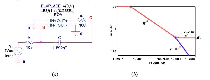
Figure 2. (a) PSpice circuit used to investigate the effect of the op amp’s nonzero output resistance \(r_o\). (b) Because of feedthrough, the high-frequency asymptote is now |\(a_{ft}\)| = 100/(10,000 + 100) ≅ –40 dB.
Feedthrough may be a problem in integrator-based filters that are meant to provide substantial attenuation in the stop band. As an example, let us reconsider the running biquad filter example of the previous article, repeated in Figure 3 but with each op-amp simulating Laplace block now equipped with a 100-Ω output resistance.
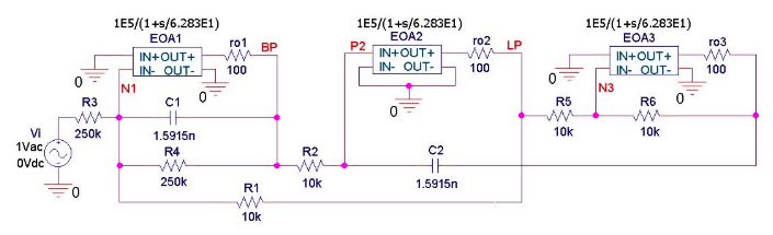
Figure 3. PSpice circuit of the biquad filter to investigate the effect of the op-amp’s output resistance \(r_o\).
As depicted in Figure 4(a), the high-frequency asymptotes of the band-pass and low-pass responses are, respectively, –68 dB and –108 dB.
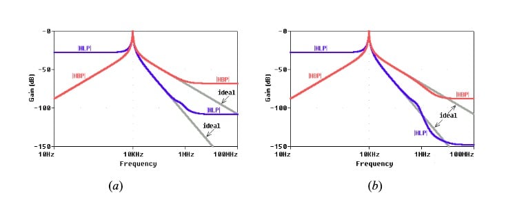
Figure 4. (a) Ac responses of the filter of Figure 3. (b) The same responses obtained either by component scaling as in Figure 5, or by using op-amps with output resistances 10 times as small.
If necessary, we can improve these figures by suitably scaling the component values. For instance, scaling as in Figure 5 (external resistances 10 times as large, capacitances 10 times as small so as to leave \(f_0\) and Q unchanged) results in the plots of Figure 4(b), where we see that the BP asymptote is lowered from –68 dB to –88 dB, and the LP asymptote from –108 dB to –148 dB.
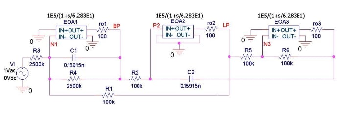
Figure 5. Component scaling by a factor of ten.
Alternatively, we can achieve the same results by using op-amps with output resistances 10 times as small (\(r_o\) = 10 Ω) while leaving the remaining components as in Figure 3.
What else would you like to learn about integrator circuits? If you want more articles like this one, tell us about your ideas in the comments below.


How to find output and input impedance of common source in software tools without simulating small signal circuit. (Note I’m using Level-1 MOSFET)[ADS Keysight].