 Facebook
 Google
 GitHub
 Linkedin
Ideal Op-Amp Characteristics
In the previous video, we discussed the basic characteristics of the operational amplifier, and we also introduced the concept of simplifying assumptions that greatly facilitate the analysis and design of op-amp-based circuits, despite the fact that they are not consistent with the electrical reality of the device.
In this video, we’ll look at five idealized op-amp characteristics. Each of the following sections will explain an idealized characteristic and compare it to the behavior that we would observe in a real op-amp. The idealized op-amp is a useful design tool, but you also need to develop the ability to identify situations in which the difference between op-amp theory and op-amp reality plays an important role in the actual performance of the circuit.
Infinite Gain
At first, this property sounds downright ridiculous. An amplifier with infinite gain will take a minuscule input signal and convert it into an infinitely large output signal. There isn’t much that you can do with an infinite output voltage, and in any case the output won’t be infinite—it is limited by the supply voltage.
In the case of an op-amp, then, infinite gain would lead to a circuit that saturates at the positive or negative rail every time a picovolt of noise creates a difference between \(V_{IN+} \) and \(V_{IN-} \).
Clearly, infinite gain isn’t very useful when the op-amp is used alone. However, we almost always use op-amps in a negative-feedback configuration, and in these situations infinite gain is indeed a very helpful assumption.
Op-amps typically have gain in the range of 10⁵ to 10⁶ V/V. Though certainly much smaller than ∞ V/V, these gains are large enough to ensure that the actual closed-loop gain of a negative-feedback circuit is very close to the theoretical value.
Infinite Common-Mode Rejection
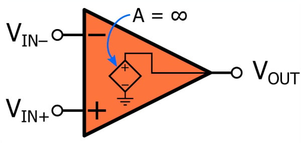
The previous video presented an op-amp as a voltage-controlled voltage source (VCVS). The control voltage for this source is (\(V_{IN+} – V_{IN–} ) \), which implies complete elimination of voltages that are present in both input signals: the only thing that affects the output amplitude is the difference between the two input amplitudes.
Infinite common-mode rejection is not realistic because it would require perfect manufacturing. However, real-life op-amps offer common-mode rejection that is high enough to meet the needs of typical applications.
Zero Input Current
We assume that no current flows into or out of the op-amp’s input terminals. Another way to express this assumption is that the op-amp has infinite input impedance.
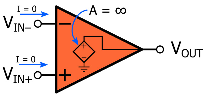
The input impedance of real op-amps is finite but usually large enough to ensure negligible amounts of current flow. Op-amps also have input bias currents—i.e., currents that flow through the input terminals and enable operation of the IC’s internal circuitry. Input bias currents are small in BJT op-amps and extremely small in MOSFET op-amps; nevertheless, they will cause serious problems in circuits that do not provide a proper DC path for these currents.
Zero Output Impedance
The VCVS op-amp model does not show any resistance that is in series with the output terminal. This indicates that the idealized op-amp has zero output impedance.
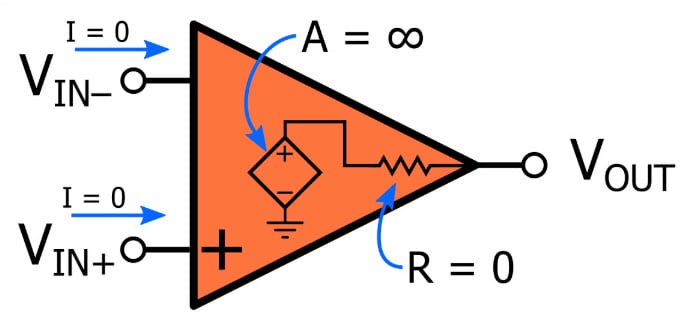
Real life op-amps have output resistance in the range of maybe 50 to 200 Ω, but the effective output resistance is greatly reduced by negative feedback. In some cases, it is appropriate to incorporate output resistance into a careful analysis of an op-amp circuit.
Infinite Bandwidth
This last idealized op-amp characteristic is the most unrealistic. The VCVS model does not contain any frequency-dependent elements, and consequently, the operation of the idealized op-amp is not affected by the frequency of the input signal. In other words, the frequency response of the op-amp would be plotted as a flat line that extends out toward infinite frequency.
This assumption is a good starting point when the goal is to understand the most basic aspects of op-amp operation, but the bandwidth of many general-purpose operational amplifiers is actually rather narrow, and real-life op-amp frequency response plays a prominent role in many design and analysis tasks. We’ll cover this important topic more thoroughly in a future video.
Summary
- An idealized op-amp exhibits various characteristics that help us to understand and implement operational amplifiers.
- These characteristics are not present in real-life op-amps, but they are reasonable approximations that often result in fully functional circuits.
- Idealized op-amps have infinite gain, infinite common-mode rejection, zero input current, zero output impedance, and infinite bandwidth.


One vexing place (rookie mistake) where the non-zero (typically 100 ohm) output impedance eats-your-lunch is where you have a lowgain amplifier (particularly with just a follower) driving a scope cable (perhaps amounting to 1000 pf) forming a RC low pass that is now directly IN THE FEEDBACK LOOP. This is often enough to destabilize unity-gain compensation, typically resulting in a small low-level (because it is slew limited) oscillation at something like 5 MHz superimposed on a typical full size audio signal; fattening (fuzzing up) the trace in an unobvious way - looking like a failure to focus the beam. [ It is only fuzzy when you measure it! ] Solution: add 1000 ohms between the op-amp output and the cable (after the intentional feedback) to get rid of the fuzzy trace.