Introduction to Reliability in Electronics: Tools and Metrics for Anticipating Device Failure

Every device fails eventually. How can you anticipate when and where issues will occur? This is where reliability engineering comes in.

Electronic products will not work forever. Whether the product is intentionally taken out of service for maintenance or stops working due to component failure—at some point, everything stops working as initially designed and produced. 

Reliability engineering uses statistical methods to provide engineers with a structured approach to system-design, estimating component and product lifetime and failure rates to determine what will fail and when.

All products have some sort of natural variation, and no manufacturing process is perfect. As an example, consider a production run of ten-thousand optocouplers. Some units will have LED emitters that are a bit brighter than others, and some units will have photo-receivers with increased sensitivity. Over time, all LEDs decrease their emitted-light output, and eventually, the dimmer emitters will fail to activate the less-sensitive receivers. At that point, the optocouplers begin to fail.

In this article, we'll take an introductory look at a few methods that allow engineers to measure and anticipate reliability issues.

 

Visualizing Failure: The Load-Strength Curve Visualization

Mechanical and electrical engineers often visualize system components with probability density functions (PDFs). These statistical curves show the natural variation in strength for a large population of components/products as well as the natural variation in load. 

Where the load and strength curves begin to overlap, failures occur.

 

This illustration of two probability density functions of two normal distributions shows the strength distribution decreasing over time. When the two curves intersect, failures appear.

 

The engineer’s job is to ensure, as much as possible, that the strength curve is far to the right of the load curve. That is because an item at the weak end of the strength curve might experience a load at the high end of the load distribution. And to make matters worse, strength curves tend to shift over time.

The safety margin for fixed strength distributions (assuming no strength loss over time) is found by finding the difference in means of the two distributions and then dividing by the square root of the sum of the squares of the standard deviations.

 

See Patrick P. O’Conner’s Practical Reliability Engineering, 5th edition, Chapter 5 for more information on load-strength interference analysis.

 

So how does one quantify reliability?

Reliability Metrics

All products fail given enough time. To get an idea of how long a particular percentage of products will survive, and how long a warranty should last, engineers often use the B_x nomenclature.

The “B” prefix is carried over from the ball-bearing industry, which initiated its usage, and the “x” details the percentage of products that fail. So, “B₁₀” is the time for 10% of the products to fail (90% remain working).

 

This survival-function graph shows the percentage of products that remain functional over time. The B₁₀, B₂₀, and B₅₀ points are shown, the times when 10%, 20%, and 50% of the products have failed.

 

The reliability survival function is used to describe the relationship between failures and time, or more specifically, the number of still-functioning products over time. This curve is created by finding the complement (1-F(t)) of the cumulative distribution function (CDF). And the CDF is the integral (area) of the PDFs shown above.

Anticipating Issues to Avoid Failure: Fault Trees

Oftentimes, though, a product will fail when any of a number of individual components or subsystems fail. Fault trees can be created to graphically represent the series of subsystem failures that can lead to overall system failure. Redundancy is built into the system with AND gates, requiring more than one subsystem to fail before causing the entire system to fail.

 

This fault tree shows that if either (subsystem A OR subsystem B) fails AND subsystem C fails, the entire system will fail.

 

The survival functions of multiple subsystems are combined to determine the system reliability, represented below by a graph.

 

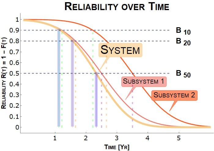
This reliability graph shows the overall system reliability of a system composed of two components, Subsystem 1 and Subsystem 2. Note from the B₁₀, B₂₀, and B₅₀ times that the overall system reliability is less than the reliability of each individual component.

 

Each additional redundant subsystem (OR) shifts the system reliability curve to the right, making the system more reliable. Every non-redundant component shifts the system reliability curve to the left, making the system less reliable over time.

---

 

This article gave a brief introduction to some of the tools and formulas reliability engineers use to learn more about a device's expected lifetime and possible failure points.

Do you have any experience in reliability engineering? Would you like to learn more about it? Leave a comment below.

Additional Resources

• The New Weibull Handbook Fifth Edition, Reliability and Statistical Analysis for Predicting Life, Safety, Supportability, Risk, Cost and Warranty Claims, Robert Abernathy, Ph.D.
• Practical Reliability Engineering, 5th Edition by Patrick P. O’Connor
• Huai Wang, Ke Ma, and F. Blaabjerg published Design for Reliability of Power Electronics Systems