 Facebook
 Google
 GitHub
 Linkedin
Using Power Spectral Density (PSD) to Characterize Noise
Learn about how power spectral density (PSD) helps us to examine the effect of a noise source on the output of a linear time-invariant (LTI) system.
Previously, we discussed that the noise PSD specifies the average power of noise at different frequencies within the bandwidth of interest. In this article, we’ll see that PSD is the main tool that allows us to examine the effect of a noise source on the output of a linear time-invariant (LTI) system.
In this article, we’ll see that PSD is the main tool that allows us to examine the effect of a noise source on the output of an LTI system.
A Transfer Function Shapes the Noise
Figure 1 shows the spectrum of a hypothetical noise source that exhibits the same average power at all frequencies, i.e. \(S_X(f)=\eta\), where η is a constant.
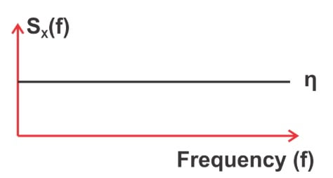
Figure 1. The spectrum of a hypothetical noise source.
If we apply this noise to an LTI system, the transfer function of the system will determine the output average power at different frequencies. For example, if the system is an ideal low-pass filter with a DC gain of 1, all of the noise frequency components in the filter stop-band will be completely suppressed. However, the frequency components in the pass band will remain unaffected (Figure 2).
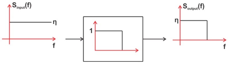
Figure 2. Example showing how the frequency components in the pass band can remain unaffected.
In general, it can be shown that the power level at a given frequency will be modified by a factor equal to the square of the magnitude of the transfer function at that frequency. This is mathematically expressed by the following equation:
\[S_{output}(f)=S_{input}(f) \times \left | H(f) \right |^2\]
Equation 1
where H(f) denotes the system transfer function. In this equation, \(S_{input}(f)\) and \(S_{output}(f)\) are the noise power spectral density in V2/Hz (not the noise voltage density in \(V/\sqrt{Hz}\)) . This equation reveals how the noise is shaped by the system transfer function.
Using this fundamental equation, we can analyze the effect of noise on the output of an LTI system.
Finding RMS Noise from the Power Spectral Density (PSD)
We know that SX(f) specifies the power of the noise waveform X in 1-Hz bandwidth around f. Since we know that, we can calculate the total noise power over a given bandwidth by calculating the total area under SX(f) in that frequency band.
For the power spectral density shown in Figure 3, the hatched area (A1) gives the total noise power in the frequency band from f1 to f2.
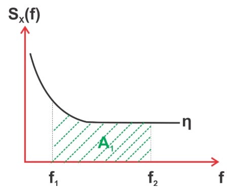
Figure 3. Example graph showing the power spectral density, where the hatched area is the total noise power in the frequency band, f1 to f2.
Let’s assume that A1 can be approximated with the area A2, as shown in Figure 4.
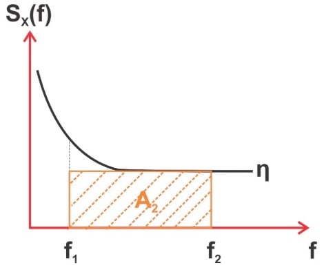
Figure 4. Similar graph as Figure 3; however, we're approximating the area of A2.
If the vertical axis in Figure 4 is in terms of \(V^2/Hz\), then the total noise power from f1 to f2 will be:
\[P_{tot}=(f_2-f_1) \eta\]
This is in terms of V2. The noise RMS (in V) can be found by calculating the square root of the above value:
\[V_{n, RMS}=\sqrt{(f_2-f_1) \eta }\]
However, manufacturers commonly specify their product noise performance by providing the square root of the PSD.
If we assume that the vertical axis in Figure 4 is in \(V/ \sqrt{Hz}\), the noise RMS (in V) will be:
\[V_{n, RMS}=\eta \sqrt{f_2-f_1 }\]
Noise Equivalent Bandwidth
For the example depicted in Figure 3, we calculated the noise power in the frequency range from f1 to f2 and completely ignored all the frequency components outside this range.
In practice, we usually need to calculate the noise power in a frequency range that is limited by the bandwidth of a filter. A real-world filter cannot have abrupt transitions from passband to stopband. Hence, we have to take into account the power of the frequency components that are in the filter roll-off region.
Figure 5 shows how a practical low-pass filter can only partially suppress the noise components in the roll-off region.
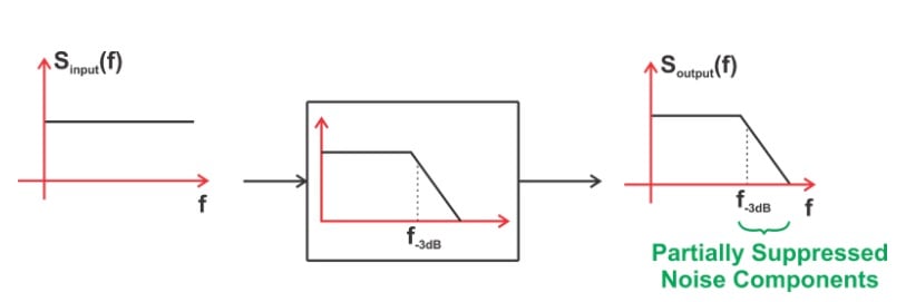
Figure 5. Example showing how a low-pass filter can partially suppress the noise components of the roll-off region.
Let’s see how we can take into account these partially suppressed components. Assume that the filter in Figure 5 is a first-order low-pass filter with the following transfer function:
\[H(f)=\frac{1}{1+j\frac {f}{f_{-3dB}}}\]
The noise spectrum at the filter output will be:
\[S_{output}(f)=S_{input}(f) \times |H(f)|^2=\eta \times \frac{1}{(1+\frac {f}{f_{-3dB}})^2}\]
The total noise power at the filter output can be found by integrating \(S_{output}(f)\) over the entire frequency range from 0 to ∞:
\[P_{tot}=\int_{0}^{\infty}\eta \times \frac{1}{1+(\frac {f}{f_{-3dB}})^2}df\]
Calculating this integral, we obtain \(P_{tot}=\eta \times \frac{\pi}{2}\times f_{-3dB}=\eta \times 1.571\times f_{-3dB}\). This is equal to the total noise power we would have if our low-pass filter had a bandwidth of \(1.571\times f_{-3dB}\) and exhibited an ideally abrupt transition from pass-band to stop-band.
Hence, to calculate the total noise power at the output of a first-order low-pass filter, we can assume that the filter roll-off is abrupt and increase the filter bandwidth by a factor of 1.571. We often refer to \(1.571\times f_{-3dB}\) as the noise equivalent bandwidth of a first-order filter that has a 3-dB bandwidth of \(f_{-3dB}\).The factor 1.571 is sometimes referred to as the shape factor.
As the filter order increases, its transition from pass-band to stop-band becomes more and more abrupt. That’s why we expect to have a smaller shape factor for higher-order filters. Table 1 below shows the shape factor for different filter orders.
| Filter Order | Shape Factor |
| 1 | 1.57 |
| 2 | 1.11 |
| 3 | 1.05 |
| 4 | 1.03 |
| 5 | 1.02 |
In the next section, we’ll see an example of using these shape factors to calculate the noise contribution from different sources in the signal chain.
Noise Bandwidth When Several Stages Are Cascaded
When we have several cascaded stages, each with a different bandwidth, we should consider the smallest bandwidth that a given noise source experiences.
As an example, consider the signal chain shown in Figure 6.
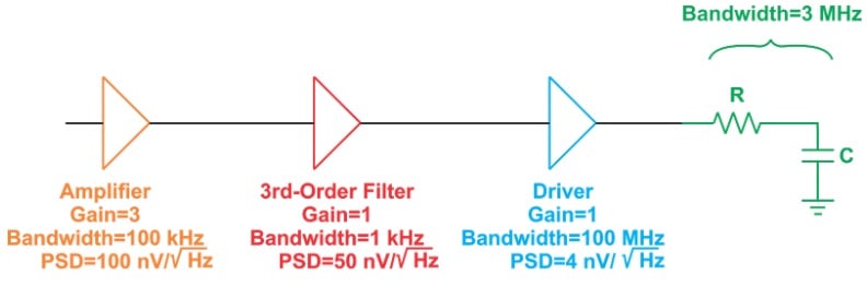
Figure 6. Example signal chain, including bandwidths, gain, and PSD.
The figure gives the gain and bandwidth for each stage. Moreover, it specifies the spectrum of the noise contributed by each stage in \(nV/\sqrt{Hz}\). The noise produced by the amplifier is \(100 nV/\sqrt{Hz}\) over the amplifier bandwidth (100 kHz). As this noise goes through the cascaded stages, its bandwidth can be further limited by the bandwidth of the different stages.
The second stage in the chain is a 3rd-order filter. Since the shape factor for a 3rd-order transfer function is 1.05, the noise bandwidth of this stage will be 1 kHz × 1.05 = 1.05 kHz. This is much smaller than the bandwidths of the driver and the RC filter, which are 100 MHz and 3 MHz, respectively. Therefore, for the noise generated by the first stage, we should consider a noise bandwidth of 1.05 kHz.
The RMS noise originating from this stage will be
\[V_{n, RMS, Amplifier}=100 nV/\sqrt{Hz} \times \sqrt {1050 Hz}=3.24 \mu V\]
Similarly, we can calculate the effective bandwidth for the other noise sources in the signal chain.
Note that a component with the highest noise spectral density is not necessarily the most dominant noise contributor to the system. For example, the amplifier PSD is several times larger than that of the driver. Because of this, one may mistakenly think that the noise contributed by the amplifier is much larger than that produced by the driver. However, this is not necessarily the case. In this example, the smallest bandwidth that the driver noise experiences are that of the RC filter.
Considering the shape factor of 1.57 for this stage, we obtain:
\[V_{n, RMS, Driver}=4 nV/\sqrt{Hz} \times \sqrt {1.57 \times 3 MHz}=8.68 \mu V\]
which is much larger than the RMS noise that originates from the amplifier.
Overview of Noise Spectral Density
- As a noise signal goes through an LTI system, its PSD gets “shaped” by the system transfer function.
- We can calculate the total power of a noise signal by calculating the total area under the PSD curve over a given bandwidth.
- To calculate the total noise power at the output of a filter, we can assume that the filter roll-off is abrupt and increase the filter bandwidth by a factor called the shape factor.
- As the order of the filter increases, its transition from pass-band to stop-band becomes more and more abrupt, and the shape factor gets closer to one.
- When we have several cascaded stages, each with a different bandwidth, we should consider the smallest bandwidth that a given noise source experiences.


Nice article. Just a two small remarks:
1. I know it is a common practice, but I think it is sloppy and confusing for newbies to say that power density is expressed in V²/Hz. I’d suggest to use the name “power density” if you have a quantity in W/Hz and calling a quantity in V^2/Hz “the squared voltage density”.
2. There is a factor missing in the formula
Ptot=f2−f1
It is als dimensionally incorrect, since P is normally expressed in W (this has of course to do with my first remark).
kind regards,
Hugo