Characterize RF Noise Components Using Equivalent Noise Temperature

Previously, we discussed that the noise figure is the commonly used noise specification in RF work. An alternative way of characterizing the noise performance of RF components and systems is the equivalent noise temperature, which will be the main focus of this article.

In general, the noise figure and equivalent noise temperature both provide the same information; however, you might be a little less familiar with the concept of noise temperature. The noise temperature is mainly used in non-terrestrial applications, such as radio astronomy and space-oriented radio links that deal with very small noise levels. Despite its niche application, familiarizing ourselves with the noise temperature concept can give us a clearer picture of how noise figure measurement instruments actually work. In fact, an automatic noise figure analyzer might perform many of its internal computations in terms of noise temperature.

 

Noise Temperature of a One-port Device: Antenna or Noise Source

We can use the noise temperature concept to specify the noise produced by a one-port device, such as an antenna or a noise source. To better understand this, consider an arbitrary white noise source with an output impedance of R connected to a matched load resistor, R_L, as shown in Figure 1(a) below.

 

Figure 1. Example diagrams of an arbitrary white noise source with an output impedance connected to a matched load resistor (a) and a single resistor at a temperature of T_e that produces the same amount of noise as the original noise source (b).

 

Let's assume that the noise source delivers a noise power of N_o to R_L = R (i.e., the maximum available noise power of the noise source is N_o). We know that the available noise power of a resistor is kTB. Equating kTB with N_o, we can find the temperature where the resistor exhibits an available noise power of N_o.

 

 \[T_e = \frac{N_o}{kB}\]

 

This observation gives us the noise model shown in Figure 1(b), where a single resistor, R, at a temperature of T_e is used to produce the same amount of noise as the original noise source, where T_e is the equivalent noise temperature of the noise source. Note that the noise temperature doesn’t indicate the physical temperature of the resistor, as you would measure it with a thermometer. The noise temperature is just a concept that allows us to model the actual noise level that a component produces. It’s also worthwhile to mention that, by definition, the noise figure concept cannot be applied to one-port devices.

 

Noise Temperature of a Two-port Device: Noisy Amplifier

The noise temperature concept can also be used to describe the noise performance of a two-port network. As an example, consider a noisy amplifier with a gain, G, and a bandwidth, B, connected to a matched source resistor, as shown in Figure 2(a).

 

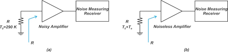
Figure 2. Example diagrams of noisy (a) and noiseless (b) amplifiers in a noise measuring system. 

 

Next, the available noise at the output of the amplifier can be described using Equation 1.

 

\[N_o = N_{o(added)} + kT_0BG\]

Equation 1.

 

Where:

• N_o(added) is the portion of the noise that is produced by the internal noise sources of the amplifier
• kT₀BG is the available noise from the source resistor (kT₀B) multiplied by the amplifier’s available power gain, G

Similar to the one-port example, we wish to model the noise from the amplifier by finding a new temperature for the source resistor. To this end, we first find the input-referred noise of the amplifier:

 

\[N_{i(added)}=\frac{N_{o(added)}}{G}\]

 

Equating the above value with kT_eB gives us the equivalent temperature where the available noise power of a resistor is equal to the input-referred noise of the amplifier in Equation 2.

 

\[T_e=\frac{N_{o(added)}}{kBG}\]

Equation 2.

 

From this, we can assume that the amplifier is noiseless and, instead, increase the initial temperature of R_s by T_e to account for the amplifier’s noise. This is illustrated in Figure 2(b).

Now, let’s verify our model by calculating the total output noise. Referring to Figure 2(b), we have:

 

\[\begin{eqnarray}
N_o &=& kTBG = k(T_0+T_e)BG \\
&=& k(T_0+\frac{N_{o(added)}}{kBG})BG \\
&=& kT_0BG +N_{o(added)}
\end{eqnarray}\]

 

Which is consistent with Equation 1 (no big surprise!). Having the noise temperature of the amplifier, T_e, we are able to find the noise temperature of the whole system, including both the source impedance, R_s, and the amplifier given by T₀ + T_e. Additionally, by combining Equation 2 with the noise factor definition below, we can obtain a useful equation that expresses the noise figure in terms of the equivalent noise temperature, shown in Equation 3.

 

\[\begin{eqnarray}
F&=& 1 + \frac{N_{o(added)}}{N_{o(source)}} \\
&=& 1 + \frac{kT_eBG}{kT_0BG} \\
&=& 1 + \frac{T_e}{T_0}
\end{eqnarray}\]

Equation 3.

 

Noise Temperature of a Cascaded System

A cascaded system made of N two-port devices is shown below in Figure 3.

 

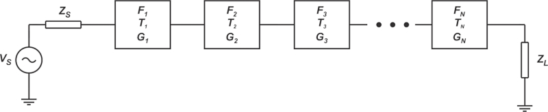
Figure 3. A cascaded system made of N two-port devices diagram.

 

Where:

• F_i is the noise factor
• T_i is the equivalent noise temperature
• G_i is the available power gain of the i-th stage

With that in mind, we know that the noise factor of the cascaded system is:

 

\[F = F_1 + \frac{F_2 - 1}{G_1} + \frac{F_3 - 1}{G_1 G_2} + \dots + \frac{F_N - 1}{G_1 G_2 \dots G_{N-1}}\]

 

Applying Equation 3, we can replace each F_i term with its equivalent noise temperature and find the noise temperature of the cascaded system:

 

\[T_{cas} = T_1 + \frac{T_2}{G_1} + \frac{T_3}{G_1 G_2} + \dots + \frac{T_N}{G_1 G_2 \dots G_{N-1}}\]

 

If T_s denotes the noise temperature of the source impedance, the noise temperature of the whole system—including R_s and the cascade—is T_s + T_cas.

Now, let’s look at a few examples to clarify the above concepts.

 

Example 1: Specifying the Noise Figure to Meet System Requirements 

Assume that for a source temperature of T_s = 60 K, the overall system noise temperature is 380 K. Find the noise figure of the cascade.

The noise temperature of the cascade itself is readily found as T_cas = 380 - T_s = 320 K. Next, we apply Equation 3 to find the required cascade noise figure:

 

\[\begin{eqnarray}
F &=& 1 + \frac{T_e}{T_0} \\
&=& 1 + \frac{320}{290}=2.1 =3.22 \text{ }dB
\end{eqnarray}\]

 

Example 2: Finding the Noise Power of a Cascaded System Output

Assume that the source noise temperature is T_s = 150 K. Also, suppose that the cascade noise factor, gain, and bandwidth are respectively F_cas = 1.8, G = 6 dB, and B = 10 MHz. Find the available noise power at the output of the cascade. 

We first use Equation 3 to find the noise temperature of the cascade:

 

\[T_{cas} = (F_{cas}-1)T_0=(1.8-1)\times 290=232 \text{ } K\]

 

Therefore, the noise temperature of the overall system is T_sys = T_s + T_cas = 150 + 232 = 382 K. Finally, we have:

 

\[\begin{eqnarray}
N_o &=& k(T_s + T_{cas})BG \\
&=& 1.38 \times 10^{-23} \times 382 \times 10 \times 10^{6} \times 10^{0.6} \\
&=& 2.099 \times 10^{-13} \text{ }W = -96.8 \text{ } dBm
\end{eqnarray}\]  

 

Revisiting the "Noise Line"—Noise Figure vs Noise Temperature

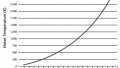
In a previous article, we looked at the plot of total output noise versus the source resistance temperature, T (Figure 4).

 

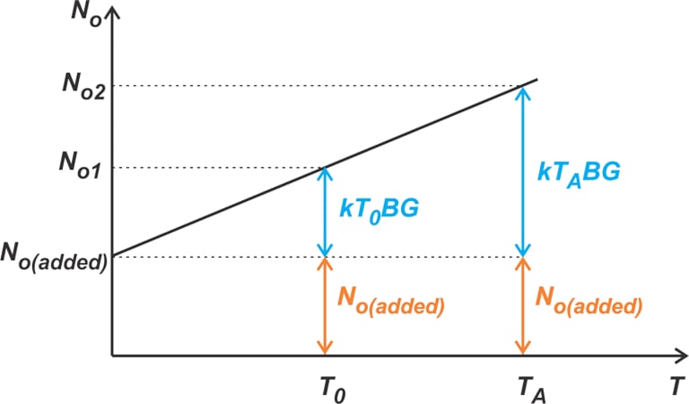
Figure 4. A plot showing the total output noise vs. the source resistance temperature.

 

This curve allows us to better understand an important difference between the noise figure and noise temperature. The noise figure metric corresponds to a standard temperature of T₀. It actually specifies the ratio of the output noise contributed by R_S at T₀ (i.e., kT₀BG) to that of the device under test, N_o(added). As can be seen from the figure, this ratio changes with T, and that’s why the noise figure is given at a standard temperature. From Equation 2, however, the noise temperature directly specifies the noise added by the device under test N_o(added), which doesn’t change with T. This feature allows us to simply add the noise temperature of a component to the arbitrary noise temperature of the source resistance; and use the overall noise temperature of the system to find the output noise power.

On the other hand, applying the noise figure concept can be a little bit tricky when the source temperature, T_s, is not the same as the standard temperature, T₀. If T_s ≠ T₀, we cannot directly use the noise figure definition to find the total output noise. In this case, we should first use the noise figure equation to find N_o(added) and then use that information to find the output noise.   

 

Noise Temperature: a Higher-Resolution Metric in Low-noise Systems

Table 1 gives the noise temperatures for some example noise figure values.

 

Table 1. Example noise temperatures for noise figure values. Data used courtesy of Thomas H. Lee

NF (dB)	F	TN (K)
0.5	1.122	35.4
0.6	1.148	43.0
0.7	1.175	50.7
0.8	1.202	58.7
0.9	1.230	66.8
1.0	1.259	75.1
1.1	1.288	83.6
1.2	1.318	92.3
1.5	1.413	120
2.0	1.585	170
2.5	1.778	226
3.0	1.995	289
3.5	2.239	359

     

Note that for very low noise systems, the noise temperature is a higher-resolution description of the noise performance. For example, while the noise figure changes from 0.5 dB to 1 dB, the noise temperature changes over a relatively larger range, from 35.4 K to 75.1 K. The noise factor also has a small change in this range, going from 1.122 to 1.259. Being a higher-resolution representation, the noise temperature is usually used in characterizing satellite communications systems that deal with exceptionally low noise levels. 

 

Antenna Noise Temperature

As the final section of this article, let’s take a brief look at some of the factors that can have an impact on the noise temperature of an antenna. The electrical model of an antenna used as a receiving element is shown below (Figure 5).

 

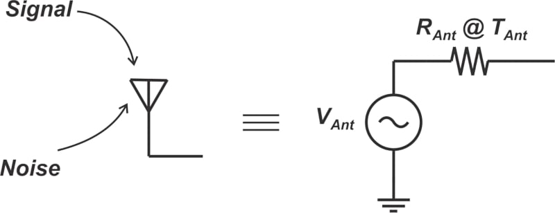
Figure 5. Diagram of an antenna used as a receiving element.

 

The voltage source, V_Ant, represents the ability of the antenna to collect signals. R_Ant actually models the matching property of the antenna that matches the characteristic impedance of free space to that of our circuitry. The antenna also picks up both signal and noise components impinging on it.

To model the collected noise, we assume that R_Ant is at a noise temperature of T_Ant. The noise the antenna picks up, and consequently T_Ant, depends on several different factors, such as the position of the antenna, its elevation angle, and frequency of interest. For example, if the antenna is oriented toward an electronic device that generates electromagnetic interference (EMI), we expect to collect a greater amount of noise power. However, repositioning the antenna away from the noise source can reduce the noise level. 

The antenna elevation off of the horizon is also an important parameter. In ground-to-ground radio links, the antenna is pointed at the horizon. Thus it picks up thermal radiation from the ground, leading to a typical noise temperature of about 290 K, which is the standard temperature used in the definition of noise figure.

On the other hand, in satellite communications, the antenna is pointed at the sky, and the equivalent noise temperature is normally much lower, typically about 50 K. That’s why satellite communications systems deal with exceptionally low noise levels and usually characterize their systems using the noise temperature metric. The antenna noise temperature also changes with frequency. Figure 6 shows the noise temperature versus the frequency for an antenna with an elevation angle of 5°.

 

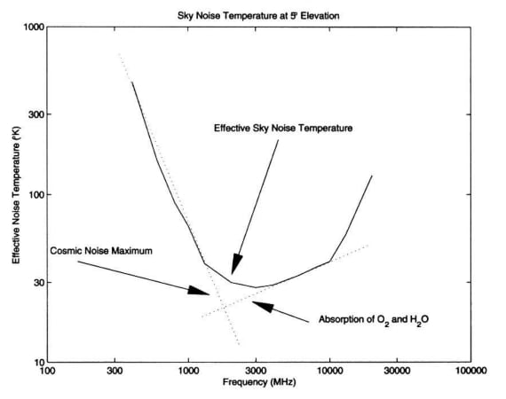
Figure 6. Plot showing the noise temperature vs. frequency for an antenna with an elevation angle of 5°. Image used courtesy of Kevin McClaning

 

Summarizing the Noise Temperature Concept

The noise figure and noise temperature are interchangeable characterizations of the noise performance. The noise temperature concept is mainly used in non-terrestrial applications, such as radio astronomy and space-oriented radio links that deal with very small noise levels. Also, familiarity with the noise temperature concept can give us a clearer picture of how noise figure measurement instruments actually work. In the next article, we’ll discuss one of the commonly used methods for noise figure measurement, namely the Y-factor method, which extensively uses the noise temperature concept.

 

---

 

To see a complete list of my articles, please visit this page.