Understanding Different Definitions of the Spurious Free Dynamic Range (SFDR) Specification

Noise and linearity performance are two of the most critical characteristics of an analog circuit. While the noise performance determines the smallest signal that the circuit can process, the circuit linearity sets an upper limit for the signal amplitude. In this article, we’ll look at the spurious free dynamic range (SFDR) which is a popular specification for quantifying the linearity of a circuit.

Modelling Nonlinearity

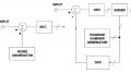
Assuming that our nonlinear circuit is memoryless (the output at any time depends only on the input at the same time), we can use the following equation to approximate the input-output characteristic: 

\[v_{out}(t)=\alpha_1v_{in}(t)+\alpha_2{v_{in}}^2(t)+\alpha_3{v_{in}}^3(t)+\alpha_4{v_{in}}^4(t)+...\]

where \(v_{in}(t)\) and \(v_{out}(t)\) are the circuit input and output signals, respectively. While the coefficient \(\alpha_1\) specifies the linear gain of the circuit, the other coefficients \(\left ( \alpha_2 , \alpha_3 ,\alpha_4 , \cdots \right )\) characterize the circuit distortion. For a fully differential circuit, the even-order distortion terms \(\left ( \alpha_2 , \alpha_4 , \cdots \right )\) are usually negligible and we have:

\[v_{out}(t) \simeq \alpha_1v_{in}(t)+\alpha_3{v_{in}}^3(t)\]

Equation 1

Note that the above equation assumes that \( \alpha_3 \) is the dominant term and ignores the higher odd-order terms \(\left ( \alpha_5 , \alpha_7 , \cdots \right )\)

Single-Tone SFDR

Assume that a single-tone sinusoid, \(v_{in}(t) \), is applied to the non-linear circuit described by Equation 1:

\[v_{in}(t)=A\cos(\omega t)\]

The output will be:

\[v_{out}(t)=\left ( \alpha_1 A + \frac {3 \alpha_3 A^3}{4} \right )cos(\omega t)+ \frac{\alpha_3 A^3}{4} cos(3 \omega t)\]

While the input is a single-tone sinusoid at \( \omega \) , we have two different components at the output: one at \( \omega \) and another one at \( 3 \omega \). This is shown in Figure 1.

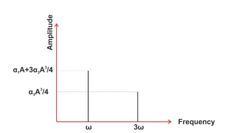
Figure 1

The component at \( \omega \) is usually the desired output; however, the component at 3\( \omega \) (often referred to as the third harmonic) is produced only because of the circuit non-linearity (non-zero \(\alpha_3\)). 

The above analysis was based on a number of simplifying assumptions. For example, we assumed that the circuit is memoryless and that the output voltage at \(t = t_0 \) is a function of the input at \(t = t_0 \). Additionally, we only considered one of the distortion terms. In the real world, these assumptions may not always be valid. As a result, a non-linear circuit may produce several frequency components at the output, although the input is a single-tone sinusoid. This is illustrated in Figure 2.

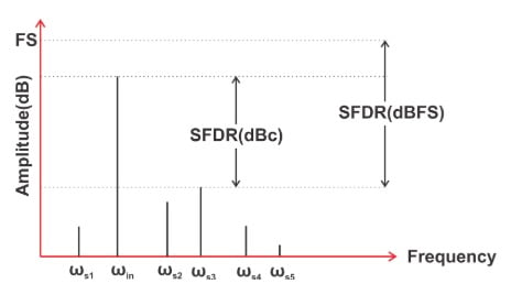
Figure 2

This figure shows the output of a hypothetical circuit with a single-tone input at \( \omega_{in} \). In addition to the desired output at \( \omega_{in} \), there are several different frequency components (spurs) in the output spectrum. The nonlinearity analysis of the previous section predicted that the produced frequency components are harmonics of the input frequency. However, in reality, the spurs may or may not be harmonically related to the input.

There are several different specifications that can be used to characterize the circuit linearity. One popular specification is the spurious free dynamic range (SFDR). The SFDR specification is defined as the ratio of the desired signal amplitude to the largest spur over the bandwidth of interest. This ratio is usually expressed in dB. Since this definition specifies the maximum spur amplitude in reference to the signal (or carrier) level, we express the SFDR in dBc (dB relative to the carrier) as depicted in Figure 2. Sometimes, we prefer to express the maximum spur level in reference to the full scale value of the circuit (dBFS). This latter unit is usually utilized when dealing with circuits such as A/D converters that have a precisely defined maximum output signal. 

Two-Tone SFDR

Assume that the following two-tone input is applied to the non-linear circuit described by Equation 1:

\[v_{in}(t)=Acos(\omega_1 t)+Acos(\omega_2 t)\]

The output will be:

\[v_{out}(t)=(\alpha_1 A+ \frac{9 \alpha_3 A^3}{4})(cos(\omega_1t)+cos(\omega_2t))\]

\[+\frac {\alpha_3 A^3}{4}(cos(3 \omega_1t)+cos(3 \omega_2t))\]

\[+ \frac{3\alpha_3 A^3}{4}(cos((2\omega_1+\omega_2)t)+ cos((2\omega_2+ \omega_1)t))\]

\[+ \frac{3\alpha_3 A^3}{4}(cos((2\omega_1-\omega_2)t)+ cos((2\omega_2- \omega_1)t))\]

While the input consists of two components at \(\omega_1\) and \(\omega_2\), we have several different frequency components at the output at \(\omega_1, \omega_2, 2\omega_1 \pm \omega_2 ,\) and \(2\omega_2 \pm \omega_1\). If \(\omega_1\) and \(\omega_2\) are close to one another, the frequency components at \(3\omega_1, 3\omega_2, 2\omega_1 + \omega_2 ,\) and \(2\omega_2 + \omega_1\) will be far away from the desired output components at \(\omega_1\) and \(\omega_2\). Hopefully, we can filter these undesired components.

However, there are two other terms at  \(2\omega_1 - \omega_2\) and \(2\omega_2 - \omega_1\) that are very close to the desired signals and cannot be easily filtered out (noting that \(\omega_1\approx \omega_2\)). Figure 3 shows the output of a non-linear circuit for a two-tone test.

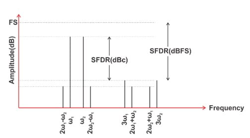
Figure 3

Figure 3 illustrates that we can define the SFDR for this test as the ratio of the amplitude of either of the two original tones to the largest spur over the bandwidth of interest. Again, we can express the SFDR in dBc or dBFS. We usually refer to the SFDR illustrated in Figure 2 as the single-tone SFDR and that defined in Figure 3 as two-tone SFDR. Similarly, we can define this specification for a multi-tone input (a multi-tone SFDR). This is shown in Figure 4.

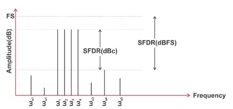
Figure 4

Note that the spurs in Figures 2, 3, and 4 may or may not be harmonically related to the input.

Noise-Related Definition of SFDR

There’s another definition for SFDR that is somewhat different from those discussed above. This definition is based on a two-tone test. As discussed above, the two-tone test creates several distortion components. The distortion components that this new SFDR definition takes into account are those at \(2\omega_1 - \omega_2\) and \(2\omega_2 - \omega_1\) that have an amplitude of \(\frac {3 \alpha_3 A^3}{4}\). The amplitude of these components are proportional to the input amplitude (A) cubed. Hence, if we increase the amplitude of the original tones by 1 dB, the amplitude of these components will theoretically increase by 3 dB. This is illustrated in Figure 5.

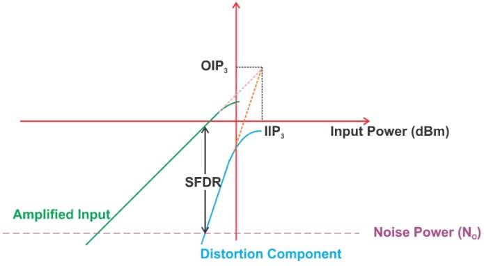
Figure 5  

This figure shows the power of the desired output and the distortion component versus the input power (all in dBm). The blue curve that shows the power of the distortion term increases with a slope of 3, whereas the green curve that shows the power of the desired output increases with a slope of one.

As the input amplitude (A) increases, the distortion component becomes larger and larger until its power becomes larger than the noise power at the output of the circuit (the purple line). The signal-to-noise ratio (SNR) when the power of distortion equals the output noise power is defined as the SFDR value. This is graphically illustrated in Figure 5. With this definition, it can be shown that the SFDR is given by

\[SFDR= \frac {2}{3}({OIP}_3-N_O)\]

where \(N_O\) is the noise power at the circuit output and \(OIP_3\) refers to the output power at the intersection of the green and blue curves. At this point, the power of the distortion component is equal to the power of the desired output. Note that this intersection point can only be found by extrapolating the corresponding curves. This is due to the fact that as the input power increases, the circuit exhibits more and more of its nonlinear behavior. As a result, the desired output and the distortion component gradually stop increasing with a slope of 1 and 3, respectively. 

It’s important to note that this definition of SFDR specifies the circuit nonlinearity for a given bandwidth because it compares the distortion component with the circuit noise power, which depends on the circuit bandwidth. This is in contrast to the SFDR definitions in Figures 2, 3, and 4 where only the amplitude of the desired output and the distortion components are important.

SFDR Definition in RF Design

In RF design, there is another definition for the SFDR that is used to characterize the linearity of a receiver. Just like the noise-related definition, this new definition of the SFDR is based on a two-tone test. The input amplitude (A) of the receiver is increased to the point where the distortion component becomes equal to the integrated noise at the receiver output. We can consider the power of this input as the receiver’s maximum tolerable signal power.

The SFDR is defined as the maximum tolerable signal power divided by the minimum tolerable signal power. The minimum power is often referred to as the receiver sensitivity \(P_{sensitivity}\) and is given by 

\[P_{sensitivity} = -174 dBm/Hz + NF + 10 log(B) + SNR_{min}\]

where NF is the receiver noise figure in dB, B is the system bandwidth in Hz, and \(SNR_{min}\) is the minimum required SNR in dB. Assuming that both the maximum tolerable signal power (\(P_{in, max}\)) and \(P_{sensitivity}\) are in dB, we have

\[SFDR= P_{in, max}-P_{sensitivity}\]

Substituting \(P_{sensitivity}\), we obtain:

\[SFDR = \frac{2(P_{IIP3}+174 dBm-NF-10logB)}{3}-SNR_{min}\]

where IIP3 is the “input third intercept point” which is illustrated in Figure 5. For more information about this final definition of the SFDR, please refer to Section 2.4.2 of this book.      

SFDR: An Important Specification for Communications Systems

The SFDR specification is particularly helpful when dealing with communications systems. For example, the single-tone definition illustrated in Figure 2 is usually used for characterizing the linearity of an A/D converter utilized in a communications system. It allows us to assess how well the ADC can simultaneously process a very small signal in the presence of a large signal. The two-tone definition can be used to analyze the effect of large interferers on the performance of a radio receiver that needs to detect a small signal. The next article in this series will take a closer look at the common applications of the SFDR specification in characterizing communications systems.

Conclusion

In this article, we looked at the different definitions of the SFDR specification. By understanding the subtle differences between these definitions, we can use this important specification with more confidence and better understand the limitations of the components used in communication systems.