Facebook
 Google
 GitHub
 Linkedin
Some Examples with AC Circuits
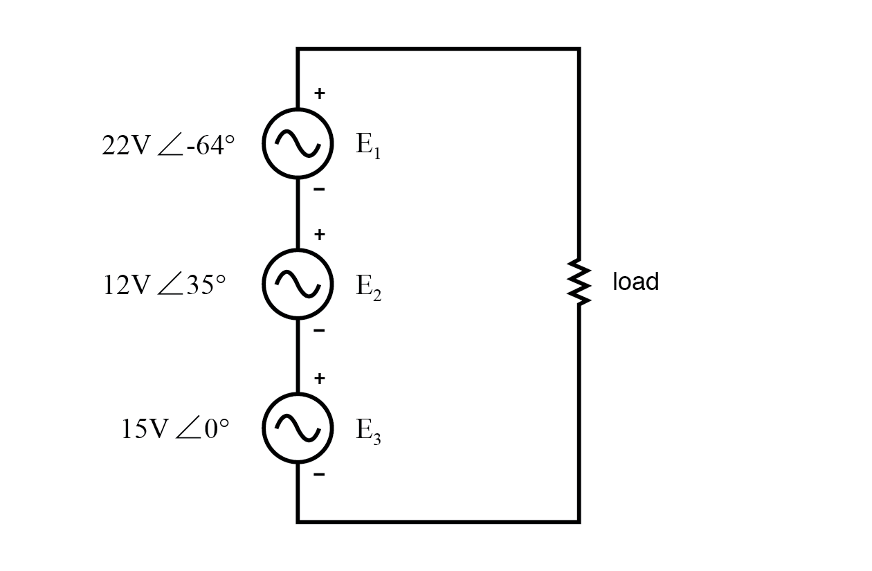
Let’s connect three AC voltage sources in series and use complex numbers to determine additive voltages.
All the rules and laws learned in the study of DC circuits apply to AC circuits as well (Ohm’s Law, Kirchhoff’s Laws, network analysis methods), with the exception of power calculations (Joule’s Law).
The only qualification is that all variables must be expressed in complex form, taking into account phase as well as magnitude, and all voltages and currents must be of the same frequency (in order that their phase relationships remain constant). (Figure below)
KVL allows the addition of complex voltages.
The polarity marks for all three voltage sources are oriented in such a way that their stated voltages should add to make the total voltage across the load resistor.
Notice that although magnitude and phase angle is given for each AC voltage source, no frequency value is specified. If this is the case, it is assumed that all frequencies are equal, thus meeting our qualifications for applying DC rules to an AC circuit (all figures given in the complex form, all of the same frequency).
The setup of our equation to find total voltage appears as such:
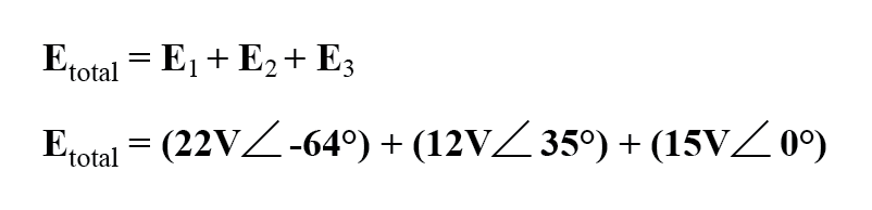
Graphically, the vectors add up as shown in Figure below.
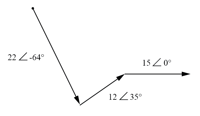
Graphic addition of vector voltages.
The sum of these vectors will be a resultant vector originating at the starting point for the 22-volt vector (the dot at upper-left of the diagram) and terminating at the ending point for the 15-volt vector (arrow tip at the middle-right of the diagram): (Figure below)
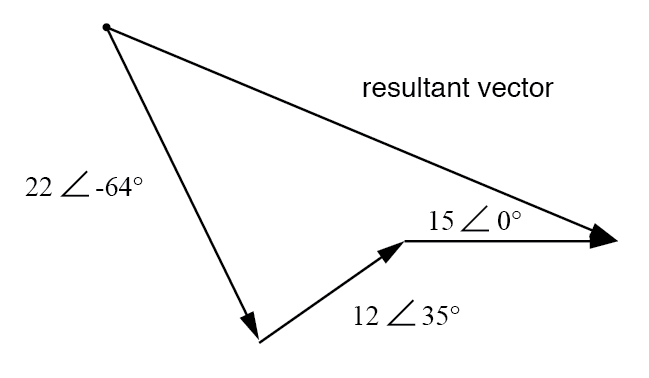
Resultant is equivalent to the vector sum of the three original voltages.
In order to determine what the resultant vector’s magnitude and angle are without resorting to graphical images, we can convert each one of these polar-form complex numbers into rectangular form and add.
Remember, we’re adding these figures together because the polarity marks for the three voltage sources are oriented in an additive manner:
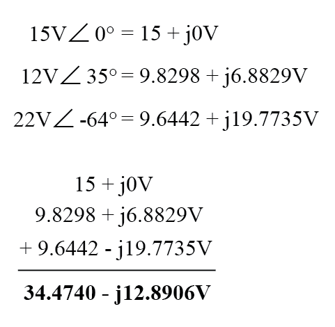
In polar form, this equates to 36.8052 volts ∠ -20.5018°. What this means in real terms is that the voltage measured across these three voltage sources will be 36.8052 volts, lagging the 15 volts (0° phase reference) by 20.5018°.
A voltmeter connected across these points in a real circuit would only indicate the polar magnitude of the voltage (36.8052 volts), not the angle. An oscilloscope could be used to display two voltage waveforms and thus provide a phase shift measurement, but not a voltmeter.
The same principle holds true for AC ammeters: they indicate the polar magnitude of the current, not the phase angle.
This is extremely important in relating calculated figures of voltage and current to real circuits.
Although the rectangular notation is convenient for addition and subtraction and was indeed the final step in our sample problem here, it is not very applicable to practical measurements.
Rectangular figures must be converted to polar figures (specifically polar magnitude) before they can be related to actual circuit measurements.
We can use SPICE to verify the accuracy of our results. In this test circuit, the 10 kΩ resistor value is quite arbitrary. It’s there so that SPICE does not declare an open-circuit error and abort analysis.
Also, the choice of frequencies for the simulation (60 Hz) is quite arbitrary, because resistors respond uniformly for all frequencies of AC voltage and current. There are other components (notably capacitors and inductors) which do not respond uniformly to different frequencies, but that is another subject! (Figure below)
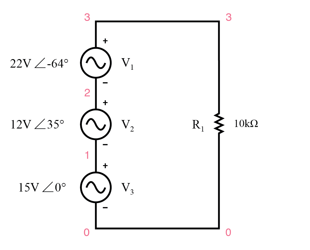
Spice circuit schematic.
v1 1 0 ac 15 0 sin
 v2 2 1 ac 12 35 sin
 v3 3 2 ac 22 -64 sin
 r1 3 0 10k
 .ac link 1 60 60            I'm using a frequency of 60 Hz
 .print ac v(3,0) vp(3,0)            as a default value
 .end
 freq           v(3)           vp(3)
 6.000E+01      3.681E+01      -2.050E+01
Sure enough, we get a total voltage of 36.81 volts ∠ -20.5° (with reference to the 15-volt source, whose phase angle was arbitrarily stated at zero degrees so as to be the “reference” waveform).
At first glance, this is counter-intuitive. How is it possible to obtain a total voltage of just over 36 volts with 15 volt, 12 volts, and 22-volt supplies connected in series? With DC, this would be impossible, as voltage figures will either directly add or subtract, depending on polarity.
But with AC, our “polarity” (phase shift) can vary anywhere in between full-aiding and full-opposing, and this allows for such paradoxical summing.
What if we took the same circuit and reversed one of the supply’s connections? Its contribution to the total voltage would then be the opposite of what it was before: (Figure below)
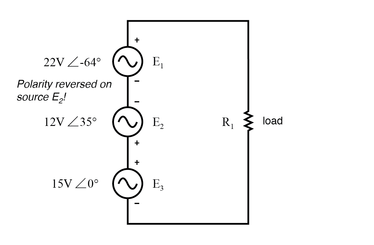
The polarity of E2 (12V) is reversed.
Note how the 12 volt supply’s phase angle is still referred to as 35°, even though the leads have been reversed. Remember that the phase angle of any voltage drop is stated in reference to its noted polarity. Even though the angle is still written as 35°, the vector will be drawn 180° opposite of what it was before: (Figure below)
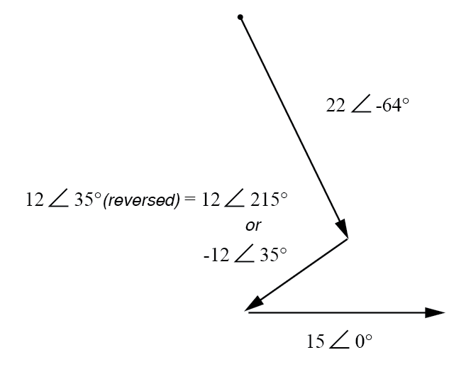
The direction of E2 is reversed.
The resultant (sum) vector should begin at the upper-left point (origin of the 22-volt vector) and terminate at the right arrow tip of the 15-volt vector: (Figure below)
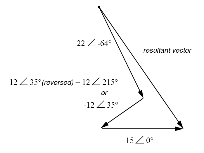
Resultant is vector sum of voltage sources.
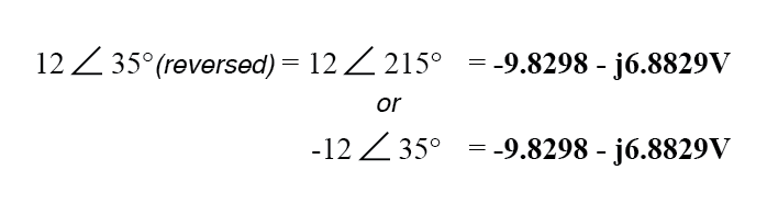
The connection reversal on the 12 volt supply can be represented in two different ways in polar form: by addition of 180° to its vector angle (making it 12 volts ∠ 215°), or a reversal of sign on the magnitude (making it -12 volts ∠ 35°). Either way, conversion to rectangular form yields the same result:
The resulting addition of voltages in rectangular form, then:
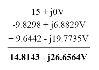
In polar form, this equates to 30.4964 V ∠ -60.9368°. Once again, we will use SPICE to verify the results of our calculations:
ac voltage addition
 v1 1 0 ac 15 0 sin
 v2 1 2 ac 12 35 sin            Note the reversal of node numbers 2 and 1
 v3 3 2 ac 22 -64 sin            to simulate the swapping of connections
 r1 3 0 10k .ac lin 1 60 60
 .print ac v(3,0) vp(3,0)
 .end
 freq           v(3)           vp(3)
 6.000E+01      3.050E+01      -6.094E+01
REVIEW:
- All the laws and rules of DC circuits apply to AC circuits, with the exception of power calculations (Joule’s Law), so long as all values are expressed and manipulated in complex form, and all voltages and currents are at the same frequency.
- When reversing the direction of a vector (equivalent to reversing the polarity of an AC voltage source in relation to other voltage sources), it can be expressed in either of two different ways: adding 180° to the angle, or reversing the sign of the magnitude.
- Meter measurements in an AC circuit correspond to the polar magnitudes of calculated values. Rectangular expressions of complex quantities in an AC circuit have no direct, empirical equivalent, although they are convenient for performing addition and subtraction, as Kirchhoff’s Voltage and Current Laws require.
RELATED WORKSHEETS: