Facebook
 Google
 GitHub
 Linkedin
Voltage-Controlled Oscillators for PLLs
How do you design a voltage-controlled oscillator? We saw some examples in the Oscillators and Timers chapter. For most applications, though, VCOs for phase-locked loops are specialized for high-frequency operation.
We have two examples here. The first (Figure 14-9) is a current-controlled oscillator, though it's a simple matter to convert the current into a voltage.
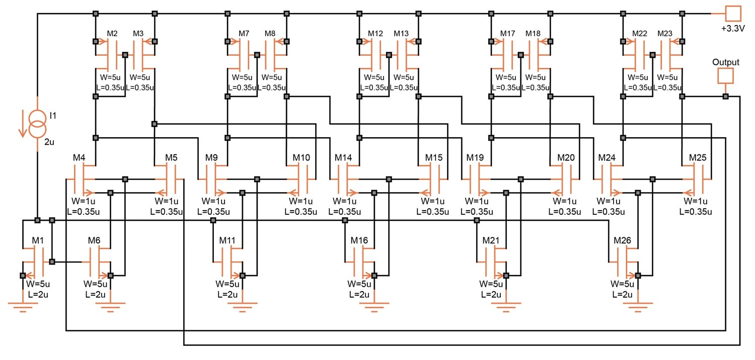
Figure 14-9. Current-controlled ring oscillator for operation between 6 MHz and 300 MHz. [click to enlarge]
Current source I1 sets the operating currents for five simple differential amplifiers with active loads. In this circuit, the output of each amplifier is connected to the input of the next stage. The output of the last stage is fed back to the input of the first amplifier. This is what's known as a ring oscillator.
The frequency of the ring oscillator is a function of the delays as the signal passes through each stage. The delays are dependent on the operating current. They increase as the operating current is decreased.
With I1 = 10 μA, the delay in each stage amounts to 1.6 ns, and the frequency is 300 MHz. With I1 = 0.1 μA, the delay increases to 83 ns and the frequency decreases to 6 MHz. This is a remarkably large range.
A number of factors contribute to the delay in each stage. Each of these factors has its own temperature coefficient. The net result is a total tempco variation that ranges from +800 ppm/°C at 0.1 μA to +200 ppm/°C at 10 μA. This temperature variation can be partially compensated by introducing an opposite tempco into the current source. This compensation is typically optimized at one operating current only.
VCO With a Schmitt Trigger
Our second example uses a different approach, as we see in Figure 14-10.
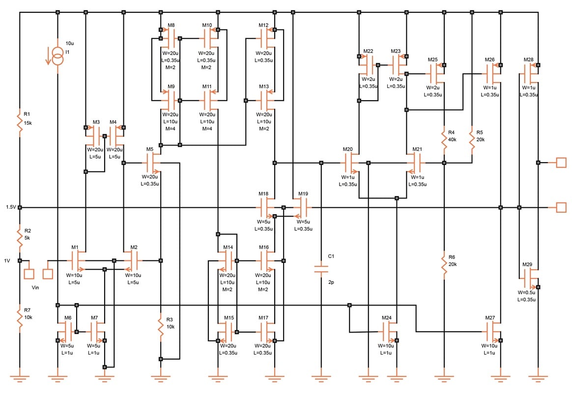
Figure 14-10. Voltage-controlled oscillator with a Schmitt trigger. [click to enlarge]
Similar to the 566 oscillator, a capacitor (C1) is charged and discharged by a current. But using two comparators and a flip-flop would be too slow for high-frequency operation, so we employ a Schmitt trigger. The Schmitt trigger has fewer devices in sequence, thus reducing delay.
There are two thresholds in Figure 14-10. The lower one is (1/2)Vdd. It's set by two equal resistors, R5 and R6. When this lower threshold is reached, M21 and M25 turn ON. This connects R4 in parallel to R5, making the upper threshold (2/3)Vdd. The resulting triangle waveform at the capacitor has an amplitude of only (1/6)Vdd peak-to-peak—we're trading accuracy for speed.
This is a somewhat improved version of a Schmitt trigger. The most important factor determining accuracy is the ON-resistance of M25. If it amounts to a substantial part of the value of R4, the effective resistance will be higher and will have a different temperature coefficient than R5 and R6.
To make this ON-resistance small, we should increase the gate width of M25. However, we can only do this at the expense of speed. The dimensions chosen for M25 are a compromise.
There is a separate stage (M26) to create a rail-to-rail swing. An inverter (M28, M29) makes both phases available to the phase detector.
The rail-to-rail output of the Schmitt trigger is also used to switch the capacitor current between charge and discharge (M18, M19). Again, the dimensions chosen here are a compromise. For accuracy over a wide control current range, we want them to be large. To get a fast response, though, they need to be small.
M1–M7 form a voltage-to-current converter; R3 is intended to be an external resistor. The control voltage is derived from Vdd through a resistor divider (R1, R2, R7) with a rest value of 1 V. The current, therefore, tracks the two thresholds, and the frequency is independent of supply voltage. With no signal at the input, the voltage-to-current converter produces 100 μA.
A large-value resistor can be inserted between the two input terminals. Then, modulating the base of M1 with the error signal changes the current by perhaps ± 10 μA or ± 20 μA.
To adapt the phase detector shown in Figure 14-2 to this VCO, an active load can be used to convert the differential error signal to a single-ended one. We would then use a current mirror to shift the error signal near ground potential.
With C1 = 2 pF, the frequency of oscillation is 36 MHz and the temperature coefficient is –370 ppm/°C. At 60 MHz (C1 = 1 pF), the temperature coefficient increases to –680 ppm/°C because of the greater role played by delay. Below 20 MHz, the temperature coefficient is close to zero.
There is a ± 0.3% change in frequency for a ± 10% change in supply voltage.