 Facebook
 Google
 GitHub
 Linkedin
Average Power Calculations of Periodic Functions
This article is following up The Effects of Symmetry on the Fourier Coefficients. Topics will cover finding the average power delivered to a resistor, calculating the RMS value of a periodic function.
Learn to calculate the average power from periodic functions
Previous articles on the Fourier series:
Learn About Fourier Coefficients
The Effect of Symmetry on the Fourier Coefficients
Calculating Average Power from Periodic Functions
Given a Fourier series representation of the current and voltage at a pair of terminals in a linear lumped-element circuit (current through and the voltage across conductors connecting elements does not vary), the average power at the terminals can be easily expressed as a function of harmonic currents as well as voltages.
By using the Fourier series theory, any periodic function wave can be reduced into a series of orthogonal functions. The sine and cosine functions of separate frequencies are orthogonal because the product of any two over the period is zero. Therefore, nonsinusoidal voltage (or current) that is not a pure sinusoidal wave can be reduced to a series of high-frequency sinusoidal harmonic functions as shown below.
$$v = V_{dc} + \sum_{n=1}^{\infty }V_{n}\cos(n\omega_{0}t - \theta_{vn})$$ Eq 1.1
$$i = I_{dc} + \sum_{n=1}^{\infty }I_{n}\cos(n\omega_{0}t - \theta_{in})$$ Eq 1.2
Each notation used Eqs 1.1 and 1.2 can be described as follows:
$$V_{dc} = $$ the amplitude of the dc voltage component,
$$V_{n} = $$ the amplitude of the nth-harmonic voltage,
$$\theta_{vn} = $$ the phase angle of the nth-harmonic voltage,
$$I_{dc} = $$ the amplitude of the dc current component,
$$\theta_{in} = $$ the phase angle of the nth-harmonic current.
By assuming that the given current's reference is in the same direction of the reference voltage drop across the terminals (finding this by using a passive sign convention), the instantaneous power (the power of any circuit at a given instant) at the terminals is vi. Now, the average power is given by:
$$P = \frac{1}{T} \int_{t_{0}}^{t_{0}+T}pdt = \frac{1}{T}\int_{t_{0}}^{t_{0}+T}vi dt$$ Eq 1.3
In order to express the average power, Eq 1.1 needs to be substituted into Eqs 1.2 and 1.3 and then integrated. Thus, Eq 1.3 can be simplified to
$$P = \frac{1}{T}V_{dc}I_{dc}t$$ integrated from $$t_{0} \rightarrow t_{0} + T$$ $$+ \sum_{n=1}^{\infty}\frac{1}{T}\int_{t_{0}}^{t_{0}+T}V_{n}I_{n}\cos(n\omega_{0}t-\theta_{vn}) \times \cos(n\omega_{0}t-\theta_{in})dt$$ Eq 1.4
By using the trigonometric identity as stated below
$$\cos\alpha\cos\beta = \frac{1}{2}\cos(\alpha - \beta) + \cos(\alpha + \beta)$$
Will simplify Eq 1.4 to
$$P = V_{dc}I_{dc} + \frac{1}{T}\sum_{n=1}^{\infty}\frac{V_{n}I){n}}{2}\int_{t_{0}}^{t_{0}+T}[\cos(\theta_{vn}-\theta_{in}) + \cos(2n\omega_{0}t-\theta_{vn}-\theta_{in})]dt$$ Eq 1.5
Finally, the second term in the integrand evaluates to zero after integrating, thus simplifying to
$$P = V_{dc}I_{dc} + \sum_{n=1}^{\infty}\frac{V_{n}I_{n}}{2}\cos(\theta_{vn}-\theta_{in})$$ Eq 1.6
The above equation 1.6 is quite significant; it states that if an interaction between a periodic current and the corresponding voltage, the total average power can be expressed as the sum of the average powers found from the interaction of currents and voltages located on the same frequency. Currents and voltages of separate frequencies do not interact to provide the average power. Thus, in these average power calculations that involve varying periodic functions, the total average power can be denoted as the superposition of the average powers associated with each harmonic current and voltage.
Finding the RMS Value of a Periodic Function
The RMS value of a series of values is the square root of the arithmetic mean (average) of the squares of the original values. The RMS value of a periodic function can be expressed in terms of the Fourier coefficients as follows:
$$F_{rms} = \sqrt{\frac{1}{T}\int_{t_{0}}^{t_{0}+T}f(t)^{2}dt }$$ Eq 1.7
Expanding f(t) to in it's Fourier series provides
$$F_{rms} = \sqrt{\frac{1}{T}\int_{t_{0}}^{t_{0}+T}\left [ a_{v} + \sum_{n=1}^{\infty}A_{n}\cos(n\omega_{0}t - \theta_{n}^) \right ]^{2}dt}$$ Eq. 1.8
The squared time function simplifies whilst integrating because the only term that comes out after integration over a period are the product of the dc term as well as the harmonic products of the same frequency. Therefore, Eq 1.8 can be simplified to
$$F_{rms} = \sqrt{\frac{1}{T}\left ( a^{2}_{v}T + \sum_{n=1}^{\infty}\frac{T}{2}A^{2}_{n} \right )}$$
$$= \sqrt{a^{2}_{v} + \sum_{n=1}^{\infty}\frac{A^{2}_{n}}{2}}$$
$$= \sqrt{a^{2}_{v} + \sum_{n=1}^{\infty}\left ( \frac{A_{n}}{\sqrt{2}} \right )^{2}}$$ Eq 1.9
This above equation expresses that the RMS value of a given function is the square root of the sum, obtained by adding together the square of the RMS value of each harmonic and the square of the dc value. For instance, assume that a periodic voltage is being represented by a finite series
$$v = 10 + 20\cos(\omega_{0}t-\theta_{1}) +15\cos(2\omega_{0}t-\theta_{2}) + 5\cos(3\omega_{0}t - \theta_{3}) + 2\cos(5\omega_{0}t - \theta_{4})$$
Then the RMS value of the voltage is given by
$$V = \sqrt{10^{2}+(20/\sqrt{2})^{2}+(15/\sqrt{2})^{2}+(5/\sqrt{2})^{2}+(2/\sqrt{2})^{2}}$$
$$= \sqrt{427} = 20.66 V.$$
A lot of the time, a periodic function requires infinitely many terms be represented by a Fourier series, and thus Eq 1.9 provides us with an estimate of the true RMS value.
Active High-Q Filters
Examine the narrowband OP amp bandpass filter as shown in Fig 1.1(a). The input to the filter illustrated in Fig 1.1(b) is known as the square wave voltage. The square wave incorporates an infinite sum of sinusoids, one at the same frequency as the square wave and the remaining sinusoids at integer multiples of that same frequency. What do you think will happen from the effect of the filter on the sum of the sinusoids?
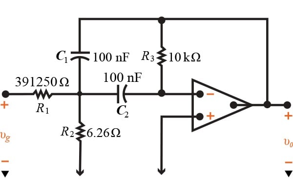
Figure 1.1 (a)
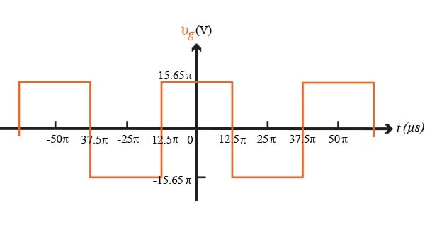
Figure 1.1 (b)
The square wave in Fig 1.1(b) can be represented by the Fourier series as follows:
$$v_{g}(t) = \frac{4A}{\pi}\sum_{n = 1,3,5,...}^{\infty}\frac{1}{n}\sin \frac{n\pi}{2}\cos n\omega_{0}t$$
In the above representation, $$A = 15.65\pi V$$. The Fourier series provides the first three terms in the equation given by
$$v_{g}(t) = 62.6\cos \omega_{0}t - 20.87\cos 3\omega_{0}t + 12.52\cos 5\omega_{0}t - ...$$
The square wave has a period of $$50 \pi \mu s$$, thus, the frequency of the square wave is 40,000 rad/s.
The transfer function (or gain) of the bandpass filter illustrated in Fig 1.1(a) is given as
$$H(s) = \frac{K\beta s}{s^{2}+\beta s + \omega^{2}_{0}}$$
Where K= 400/313, $$\Beta = 2000$$ rad/s, and $$\omega_{0} = 40,000$$ rad/s. To find the quality factor of this filter, we can divide the frequency by the Beta value, producing 40,000/2000 = 20.
By multiplying each term in the Fourier series representation of the square wave, by the transfer function H(s) evaluated at the frequency in the Fourier series gives the representation of the output voltage of the filter as a Fourier series.
$$v_{g}(t) = -80\cos \omega_{0}t - 0.5 \cos 3\omega_{0}t + 0.17 \cos 5\omega_{0}t - ...$$
After this, we need to make some changes to the bandpass filter. Letting $$R_{1}=391.25 \Omega , R_{2}= 74.4 \Omega , R_{3}=1 k \Omega,$$ and $$C_{1}=C_{2}=0.1 \mu F$$. The transfer function for the filter has the same form as $$v_{g}(t)$$, but now K = 400/313, $$\beta = 20,000$$ rad/s, and $$\omega_{0} = 40,000$$ rad/s. This bandpass gain and center frequency are unchanged, however the bandwidth is increased by a factor of 10. This change brings the quality factor to a value of 2, and the resulting bandpass filter is now less selective than the original filter! This can be seen by looking at the voltage output of the filter as a Fourier series given by:
$$v_{0}(t) = -80 \cos \omega_{0}t - 5 \cos 3\omega_{0}t + 1.63 \cos 5\omega_{0}t - ...$$
The input's fundamental frequency has the same amplification factor, but now the higher harmonic components have not been reduced as significantly as they once were when the filter with a value of Q = 20 was being used. The figure below, Fig 1.2 (a) depicts the first three terms of the Fourier series of the input square wave. Figure 1.2 (b) illustrates the first three terms of the Fourier series of the output from the bandpass filter where Q = 20. Lastly, Figure 1.2 (c) illustrates the first three terms of the Fourier series but with component values changed to provide Q = 2.
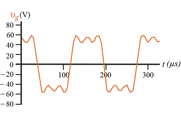
Figure 1.2 (a)
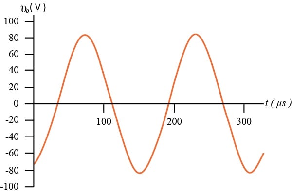
Figure 1.2 (b)
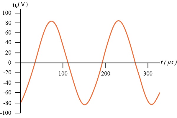
Figure 1.2 (c)
Summary
By now, you should have a good understanding of what the average power of a periodic function looks like, as well as how to calculate it. Also, you should have an understanding of the root mean square value of a periodic function. Finally, the practical application was a bandpass filter in an amplifier that was illustrated to provide a better understanding of what the periodic functions are used for. This is the last article in a series that talked all about Fourier series, I hope you have enjoyed these articles and have benefited from a better understanding of what they can be used for. If you have any questions or comments, please leave them below.
Related Content


can you post it in the PDF format so that it can be printed and saved?
thanks, Jack
My browser is showing “Math processing error”. I am actually very interested in this article. Is it possible to have it in another format or to rectify the error? Many thanks :o)