 Facebook
 Google
 GitHub
 Linkedin
Sinusoidal Steady-State Power Calculations
Let's delve into AC power concepts, how to calculate instantaneous power, average power, reactive power, complex power, and the power factor. We'll also talk about the relationship each concept has to one another.
Instantaneous Power
We begin our exploration of sinusoidal power calculations with the genaric circuit in Fig. 1.1. In here, v and i are steady-state sinusoidal signals. By using the passive sign convention (PSC), the power at any instant of time is given by:
$$p=vi$$ (1.1)
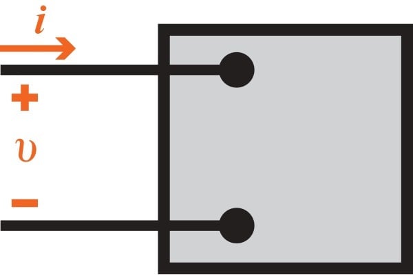
Figure 1.1 Representation of a circuit used for calculating power.
Equation 1.1 describes instantaneous power. Recall that if the reference direction of the current is in the direction of the voltage rise, Eq. 1.1 must be written with a minus sign. Instantaneous power is always measured in watts when the voltage is measured in volts and the current is measured in amperes. Two expressions of phase angles of v and i are written as
$$v=V_{m}\cos (\omega t + \theta _{v}),$$ (1.2)
$$i=I_{m}\cos (\omega t + \theta _{i}),$$ (1.3)
In these two expressions, $$\theta _{v}$$ is the voltage phase angle, and $$\theta _{i}$$ is the current phase angle.
While working in the sinusoidal steady state, a convenient reference for zero time may be chosen. Engineers who design systems that transfer large amounts of power have found it convenient to use a zero time that corresponds to the instant the current is passing through a positive maximum. By choosing such a reference time, a shift of both voltage and current by $$\theta _{i}$$ is required. Now, Eqs. 1.2 and 1.3 become
$$v=V_{m}\cos (\omega t + \theta _{v} - \theta _{i})$$ (1.4)
$$i= I_{m}\cos (\omega t)$$ (1.5)
If Eqs. 1.4 and 1.5 are substituted into Eq. 1.1, the expression for the instantaneous power now becomes
$$p= V_{m}I_{m}\cos (\omega t + \theta _{v} - \theta _{i})\cos (\omega t)$$ (1.6)
Eq. 1.6 can be used to solve for average power the way it is; however, by applying a few simple trigonometric identities the instantaneous power equation can be simplified. Using cosine's product identity gives
$$\cos (\alpha )\cos (\beta)=\frac{1}{2}\cos (\alpha -\beta )+\frac{1}{2}\cos (\alpha +\beta )$$
Letting $$\alpha =\omega t+\theta _{v}-\theta _{i}$$ and $$\beta =\omega t$$ provides
$$p=\frac{V_{m}I_{m}}{2}\cos (\theta _{v}-\theta _{i})+\frac{V_{m}I_{m}}{2}\cos (2\omega t+\theta _{v}-\theta _{i})$$ (1.7)
Lastly, using the cosine angle-sum identity
$$\cos (\alpha +\beta )=\cos (\alpha )\cos (\beta )-\sin (\alpha )\sin (\beta )$$
to expand the second term on the right-hand side of Eq 1.7, which gives
$$p=\frac{V_{mI_{m}}}{2}\cos (\theta _{v}-\theta _{i})+\frac{V_{m}I_{m}}{2}\cos (\theta _{v}-\theta _{i})\cos (2\omega t) -\frac{V_{m}I_{m}}{2}\sin (\theta _{v}-\theta _{i})\sin (2\omega t)$$ (1.8)
Relationship Between Current, Power, and Voltage
Figure 1.2 below depicts the relationship between i, v, and p, assuming that $$\theta _{v}=60^{\circ}$$ and $$\theta _{i}=0^{\circ}$$. The frequency of the instantaneous power is twice the frequency of the current or voltage. This depiction also follows from the second two terms on the right side of Eq. 1.8. This means that the instantaneous power goes through two complete cycles for every cycle of either the current or the voltage. If you look at Fig. 1.2, the instantaneous power can be negative for a portion of each cycle, even if the network between the terminals is passive. In a passive network, this negative power implies that the energy being stored in the inductors or capacitors is now being extracted. While the instantaneous power varies with time in the sinusoidal steady-state of a circuit, this causes some vibration in some motor-driven appliances. Due to this vibration in these appliances, resilient motor mountings are required to reduce any excessive vibration.
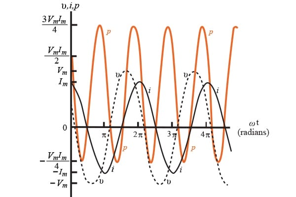
Figure 1.2 Instantaneous power, current, and voltage vs. angular frequency
Average and Reactive Power
Eq. 1.8 can now be utilized to find the average power at the terminals of the circuit, as well as establish the concept of reactive power. Noting that the equation has three terms, it can be rewritten as
$$p=P+P\cos (2\omega t)-Q\sin (2\omega t),$$ (1.9)
Where
Average (real) power $$P=\frac{V_{m}I_{m}}{2}\cos (\theta _{v}-\theta _{i})$$ (1.10)
Reactive power $$Q=\frac{V_{m}I_{m}}{2}\sin (\theta _{v}-\theta _{i})$$ (1.11)
P is called the average power, and Q is called the reactive power. Average power is also known as real power, because it is the actual power in a circuit that is transformed from electric to nonelectric energy. The average power associated with sinusoidal signals is the average of the instantaneous power over one period, or
$$P=\frac{1}{T}\int_{t_{0}}^{t_{0}+T}pdt,$$ (1.12)
Where T is the period of the sinusoidal varying function. The bounds of the integral indicate that integration can be made at any convenient time $$t_{0}$$ and integration must be bounded exactly one period later. To grasp a better understanding of all the terms in Eq. 1.9 and the relationships they hold, we will need to examine the power in circuits that are purely resistive, purely inductive, and purely capacitive.
Purely Resistive Circuits
If a circuit between terminals is purely resistive, the current and voltage are in phase $$(\theta _{v}=\theta _{i})$$. Thus, Eq. 1.9 can be reduced to
$$p=P+P\cos (2\omega t)$$ (1.13)
This is referred to as the instantaneous real power. Figure 1.3 is a graph of the instantaneous real power for a purely resistive circuit, assuming $$\omega = 377 \mathrm{ rad/s}$$. The average power, P, is the average of p, over one period. This can be seen by looking at the graph where P=1 for the circuit. From the Fig 1.3, instantaneous real power can never be negative; in other words, power cannot be removed from a purely resistive network. While the power cannot be removed, it is however, dissipated in the form of thermal energy.
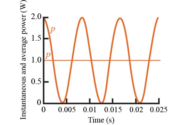
Figure 1.3 Instantaneous real power and average power of a purely resistive circuit
Purely Inductive Circuits
Now, if the circuit between the terminals is purely inductive, the current and voltage are out of phase by $$90^{\circ}.$$ The current of the circuit lags the voltage by $$90^{\circ}$$ $$(\theta _{i}=\theta _{v}-90^{\circ}).$$ The instantaneous power equation can be reduced to
$$p=-Q\sin (2\omega t)$$ (1.14)
In this purely inductive circuit, the average power is zero. This means that no transformation of energy from electric to nonelectric energy takes place. The power at the terminals is continually exchanged between the circuit and the power source driving the circuit at a frequency of $$2\omega .$$ What this means, is that when p is positive, energy is stored in the magnetic fields associated with the inductive elements, and when p is negative, energy is being removed from the magnetic fields.
Power associated with purely inductive circuits is known as the reactive power Q. Reactive power comes from the characterization of an inductor as a reactive element. To differentiate between average power and reactive power, units watt (W) for average power and var (volt-amp reactive, or VAR) for reactive power are used. Figure 1.4 depicts the instantaneous power for a purely inductive circuit, assuming $$\omega =377 \mathrm{ rads/s}$$ and Q = 1 VAR.
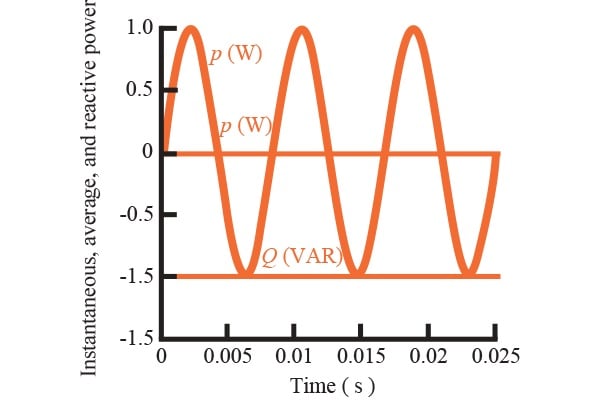
Figure 1.4 Instantaneous real power, average power, and reactive power for a purely inductive circuit
Purely Capacitive Circuits
In this purely capacitive circuit, the current and voltage are $$90^{\circ}$$ out of phase with each other. In this case, the current leads the voltage by exactly $$90^{\circ}$$ $$(\theta _{i}=\theta _{v}+90^{\circ})$$. The expression of this instantaneous power is given by
$$p=-Q\sin (2\omega t)$$ (1.15)
In this circuit, there is no transformation of energy from electric to nonelectric energy because the average power is zero. In a purely capacitive circuit, the power is continually transferred between the source delivering power and to the electric field associated with the capacitive elements. Figure 1.5 depicts the instantaneous power for a purely capacitive circuit, assuming $$\omega =377 \mathrm{ rads/s}$$ and Q = -1 VAR.
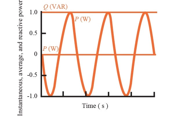
Figure 1.5 Instantaneous real power and average power for a purely inductive circuit
Understanding the Power Factor
This angle $$(\theta_{v}-\theta _{i})$$ has a significant role in computing both the average and the reactive power and is known as the power factor angle. Taking the cosine of this angle gives what is known as the power factor, shortened to pf, and taking the sine of this angle is known as the reactive factor, shortened to rf. This can be denoted as:
$$\mathrm{pf}=\cos (\theta _{v}-\theta _{i})$$ (1.16)
$$\mathrm{rf}=\sin (\theta _{v}-\theta _{i})$$ (1.17)
To completely describe the power factor angle, either lagging power factor or leading power factor terms are used. If the power factor lags, the current lags voltage (i.e. an inductive load is present). On the other hand, if the power factor leads, the current leads voltage (i.e. a capacitive load is present).
Calculating AC Power Concepts
A load comprising a 480 $$\Omega $$ resistor in parallel with a $$\frac{5}{9}\mu F$$ capacitor is connected across the terminals of a sinusoidal varying voltage source $$v_{g}$$, where $$v_{g}=240\cos (5000t) \mathrm{ V}$$
A) What is the peak value of the instantaneous power delivered by the power source?
$$P=(\frac{V_{m}}{\sqrt{2}})^{2}(\frac{1}{R})$$
$$=\frac{(240)^{2}}{2\cdot 480}$$
$$=60 \mathrm{ W}$$
Calculating the capacitive reactance:
$$X_{C}=\frac{1}{\omega c}$$
$$=\frac{-9000}{25}$$
$$=-360 \Omega $$
Calculating reactive power gained by the source:
$$Q=(\frac{V_{m}}{\sqrt{2}})^{2}(\frac{1}{X_{C}})$$
$$=\frac{(240)^{2}}{2\cdot (-360)}$$
$$=-80 \mathrm{ VAR}$$
Calculating the peak value of instantaneous power delivered:
$$p_{max}=P+\sqrt{P^{2}+Q^{2}}$$
$$=60 + \sqrt{(60)^{2}+(80)^{2}}$$
$$p_{max}=160 \mathrm{ W}$$
B) What is the peak value of the instantaneous power absorbed by the source?
$$p_{min}=P-\sqrt{P^{2}+Q^{2}}$$
$$=60-\sqrt{(60)^{2}+(80)^{2}}$$
$$p_{min}=-40 \mathrm{ W}$$
C) What is the average power delivered to the load?
Using the power equation from part A, $$= \frac{(240)^{2}}{2\cdot 480}$$
The average power is $$P= 60 \mathrm{ V}$$
D) What is the reactive power delivered to the load?
Using the reactive power equation in part A, $$=\frac{(240)^{2}}{2\cdot (-360)}$$
$$=\frac{(240)^{2}}{2\cdot (-360)}$$
$$Q=-80 \mathrm{ VAR}$$
E) Is the load absorbing or generating magnetizing vars?
Using the reactive power equation from part A, $$=\frac{(240)^{2}}{2\cdot (-360)}$$
$$Q=-80 \mathrm{ VAR}$$ A negative value means that the load is generating magnetizing vars.
F) What is the power factor?
Using the power factor equation, $$=\frac{V}{R}+\frac{V}{X_{C}}$$
$$I=\frac{240}{480}+\frac{240}{-j360}$$
$$=0.836\angle 53.267^{\circ}\mathrm{ A}$$
Therefore, the power factor is $$pf=0.6$$ leading
G) What is the reactive factor?
Using the reactive factor equation, $$\sin (0^{\circ}-53.267^{\circ})$$
Therefore, the reactive factor is $$rf=-0.8$$


Good elaboration, refreshes my school time!
Found 1 typo: “The average power is P=60V”
This is an interesting read. I have some questions however; Can you provide references and reasoning for shifting the current angle to time zero for the instantaneous power derivation, and also provide references for uses of the “rf” reactive factor terminology? Thanks.
CAPTION ERROR: Figure 1.5 Instantaneous real power and average power for a purely ‘INDUCTIVE’ circuit. Should be ‘CAPACITIVE’