Facebook
 Google
 GitHub
 Linkedin
Better Insight into DSP: 10 Applications of Convolution in Various Fields
This article presents an overview of various applications which exploit convolution, an advanced signal operation.
This article presents an overview of various applications which exploit convolution, an advanced signal operation.
Background
The background information which will help you understand this article is presented in Better Insight into DSP: Learning about Convolution. This current article expands upon the convolution topic by describing practical scenarios in which convolution is employed.
Technically, there are 12 applications of convolution in this article, but the first two are explored in my first article on the subject. These two applications are:
- Characterizing a linear time-invariant (LTI) system in terms of its transfer function
- Determining the output of an LTI system when its input is known
Again, you can learn more about these applications in the link supplied above. Now, let's move on to learning how convolution is applied in various fields.
1. Image Processing
Image processing in spatial domain is a visually rich area of study dealing with pixel-manipulation techniques. Different operations are performed over the images, which are treated simply as two-dimensional arrays.
Normally, all these matrix-based operations are performed between a larger matrix (representing the complete image) and a smaller matrix (which is known as a 2D kernel). The kernel size and the associated values determine the impact exerted by it on the image considered.
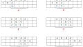
For example, suppose we have a matrix [0 1;-1 0] and convolve it an image as seen in Figure 1(a); the result will be like the one shown in Figure 1(b). We can see that the convolving operation has led to the determination of edges prevalent in the figure. However, the result obtained is incomplete because we don't yet have the complete set of edges.
In order to get the remaining set of edges, we need to perform the convolution operation once more. But this time our kernel will be [0 -1;1 0] instead of [0 1; -1 0]. The edges resulting from this are as shown in Figure 1(c).
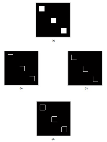
Figure 1. (a) Original image (b) First set of edges in the image (c) Second set of edges in the image (d) Edges of the original image.
Following this, we need to combine the results of both operations above to attain all of the edges present in the image (Figure 1(d)). The pair of kernels mentioned are named as Roberts’ kernels and the entire act performed on the original image is known as Roberts’ edge detection.
On the other hand, if the kernel sized 3×3 with a value of 1/9 for every element, then its convolution with an image smoothes the image, as shown in Figure 2. That is, the resultant image will be less noisy in comparison with the original one. The operation is known as smoothing and the kernel is called a smoother.
.jpg)
Figure 2. Smoothing operation.
In either of the examples here, we see a common factor—“convolution”. Convolution has more image processing applications beyond these examples and is considered important for image-processing operations.
2. Synthesizing a New Customizable Pattern Using the Impulse Response of a System
Consider a system whose impulse response (the output of the system for a unit impulse input) is as shown in Figure 3(a). Now, suppose that we want this pattern to appear at the time instant t = 25.
To accomplish this, we would need to have an input signal which has an impulse at t = 25. The presence of an impulse at the input of the system (“first impulse” shown in Figure 3(b)) results in the appearance of the system’s impulse response at that particular time instant (shown as “first impulse response” in Figure 3(c)).
If we want our impulse response to appear at t = 175 after being scaled by a factor of 1.8, then we need to have an impulse scaled by the same amount present at t = 175 on the input side.
Taking this a step further, let's say we want to invert it at t = 275. Then we'd need to have an inverted impulse at the same time instant. The associated waveforms are shown by the second set of impulses and the associated responses of Figures 3(b) and 3(c), respectively.
Figure 3. Customizing the required pattern using impulse response of the system
On the same grounds, we can guess that if we wish to have a train of this system’s response with a spacing of, say, t = ‘a’ units, then, we can get it just by exciting the system by an impulse train whose spacing is also of ‘a’ time units.
However, a word of caution about inter-impulse spacing. For faithful replication, sufficient spacing between the samples must be ensured or else distortion sets in.
For example, if the impulse response of the system spans for a duration of ‘s’ time units, then the spacing between the samples in the input signal must be greater than or equal to ‘s’ units of time. Anything less than this would lead to overlapping samples, which would affect the output. This can be observed in the last part (the third set) of Figure 3(c), which shows distorted output as the impulse train (shown as third set of impulses in Figure 3(b)) is spaced at the intervals of 30 time instants while the impulse response (in Figure 3(a)) itself spans for about 75 time units.
The illustration indicates that we can synthesize a customized output pattern by employing convolution, provided it only requires the repeating system’s response either in a scaled or unscaled fashion.
3. Signal Filtering
Let's check out the equation of a digital domain FIR (finite impulse response) filter:
$$ y[n] = \sum_{k=0}^Nh[k]x[n-k] $$
where y[n] is the output obtained by passing an input signal x[n] through a filter whose coefficients are h[n].
Here, the limits of summation range from 0 to N as our h[n] signal is finite in nature.
However, notice that even if we were to change our limits beyond this range, it would leave the filter unaffected. Suppose we took the summation from k = -2 to N + 5 (instead of 0 to N). Even then, our output remains the same. This is because the value of h[n] for k = -2 to 0 and for N to N + 5 will be zero, meaning that the summation would also be zero.
Generalizing this, we can even write the equation of FIR filter (just for convenience) as
$$ y[n] = \sum_{k=-\infty}^{\infty}h[k]x[n-k] $$
Take a closer look. Does this seem familiar to you? You may recognize this as the equation of digital convolution (as discussed in Part I).
What does this mean? Are filtering and convolution same? The answer is ‘yes’—provided that our impulse response function is same as the filter function.
The same kind of analogy holds good even when we consider the IIR (infinite impulse response) filters. However, there's an exception in that this time we need to convolve both the input as well as the past output signals with their respective coefficients.
Put simply, convolution forms a base (even in the case of 2-D images) on which signal filtering triumphs.
4. Polynomial Multiplication
Consider a case where we want to multiply two polynomials, say, (2x2 + 3x – 1) and (3x3 – 2x). The work used to achieve this result is shown below
(2x2 + 3x – 1) × (3x3 – 2x) = 6x5 - 4x3 + 9x4 - 6x2 - 3x3 + 2x
= 6x5 + 9x4 - 7x3 - 6x2 + 2x
Equation 1.
Now, let's form two arrays whose elements are the coefficients of the polynomials mentioned and then convolve them. In this example, the arrays would be array 1 = A1 = {2, 3, -1} and array 2 = A2 = {3, 0, -2, 0}.
We'll convolve them as shown in Table 1 by using a multiply-and-add technique, which you can read about in Part I of this article series.
From the table, their convolved result is {6, 9, -7, -6, 2, 0}. Expressed in its polynomial form, this is equivalent to what's shown in Equation 1.
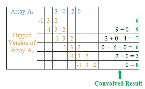
Table 1.
The resultant table indicates that, when we are multiplying two polynomials, we are actually convolving their coefficients from a mathematical perspective. This neatly demonstrates that convolution aids us in performing the multiplication of polynomials.
5. Audio Processing
Auditoriums, cinema halls, and other similar constructions heavily rely on the concept of reverberation because it enhances the quality of sound greatly.
The process in which reverberation is digitally simulated is technically termed "convolution reverb". With convolution reverb, you can convolve an area's known impulse response with that of a desired sound in order to simulate the reverberation effect of a particular area.
Here's something cool we can do with such a simulation: We can figure out the effect of an auditorium's acoustics on a violinist's performance without being present there physically. Yet another way of using this technique is to merge two sounds—say, the voice of a singer with that of a veena, to produce a new sound.
6. Artificial Intelligence
Neural networks is an area of artificial intelligence which designs circuits by imitating connections in a human brain. The interconnection between neurons within the brain is modeled as the interconnection between the nodes of multiple layers constituting a network.
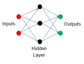
Figure 4. A simple artificial neural network
Figure 4 shows such an artificial neural network (ANN) in its simplest form. The example has a single hidden layer which routes the input nodes to the output nodes. The nodes are shown as circular regions while the blue lines indicate the interconnections.
In such a network, each interconnection is associated with a parameter called a weight. These weights indicate how much a particular node influences a particular output. Some neural networks also incorporate convolution—they are known as convolutional neural networks and they are powerful tools for image processing.
7. Synthesized Seismographs
Seismology is a branch of geophysics primarily concerned with the study of earthquakes and other cases of elastic waves traveling through the earth or even other planets. Seismic waves can travel through different layers of earth, each with its own composition and reflectivity. A net reflected wave can be obtained by summing up all reflected waves. The resulting graph is technically termed as a "synthetic seismogram".
The act of multiplying reflection coefficients of particular earth layers with an incoming signal and then summing the resultant waves can be effectively modeled via convolution operation. In other words, we can say that the reflectivity series of the earth, which can be thought of as analogous to the earth’s impulse response, can render a synthetic seismogram when convolved with the incoming seismic wave (Seismic Modelling and Pattern Recognition in Oil Exploration).
8. Optics
When collimated light passes through an aperture with a slit in it, the light gets diffracted along the discontinuity. This act results in the formation of a sinc function on the plane placed at infinity which is referred to as the diffraction pattern of light passing through the slit. Likewise, for a circular aperture, the resulting diffraction pattern would be a sombrero function (Introduction to Imaging Spectrometers).
Now, suppose that we have an aperture which is a combination of both of these (slits and circular shapes). Can we arrive at the diffraction pattern of this complex structure without actually repeating the process? Yes, we can. In fact, the resulting pattern will be the pattern obtained by convoluting the sinc function with that of sombrero.
This indicates that, when we know the diffraction patterns for each kind of aperture, the diffraction pattern of a combination of them can be obtained by convolving these individual patterns. A similar kind of superposition-like behavior is exhibited by most of the linear systems that convolution can help simplify.
9. Probability Theory
Let's consider a situation where we have two independent random variables, X and Y, with probability density functions (pdfs) f and g respectively. If we wish to compute the pdf of their sum (i.e., if we need the pdf of X + Y ), we can use the convolution of f and g.
Continuing with this logic, we can compute the pdfs of the summation of any number of independent variables. This is important because many of the standard distributions are characterized by simple convolution patterns, which means that we can find their pdfs using convolution.
10. Computed Tomography
Tomography is a technique of obtaining a particular planar view of an object. A narrow beam of x-rays (or any other similar penetrating radiation) produced from a source is made to pass through the desired object. These rays are then collected by detectors usually placed on the other side of the object.
The resulting image is the convolution of the source rays with the composition of the object, revealing its internal structure. However, the quality of the resulting image is relatively low.
Now consider a case wherein the source and the detector assembly are translated along different angular positions across the object. This act creates multiple views of the object across the same intended plane. Next, these views are acted upon by CT reconstruction algorithms so as to obtain a high-quality image.
Convolution comes in at this point where reconstruction algorithms are used. Amongst the two most widely used reconstruction algorithms is filtered back projection, which makes use of convolution.
Conclusion
This article discusses the use of convolution operation in various fields with the goal of highlighting its importance. Please feel free to share other uses of convolution in the comments below.