Facebook
 Google
 GitHub
 Linkedin
Better Insight into DSP: Learning about Convolution
This article presents an overview of the convolution operation and discusses two of its applications.
This article presents an overview of the convolution operation and discusses two of its applications.
Background Information
The world is increasingly streaming with electronic gadgets, a few for necessity but most for luxury. Irrespective of the category to which they fall-into, we can notice the basic fact that all of them make use of ‘signals’ to accomplish their tasks.
Now, is it just enough to have signals? No, absolutely not. When we have signals, at some point of time, we will, for sure, come-up with a need to process them. All such signal manipulating operations can be grouped under a common but a very broad branch named “Signal Processing”.
Depending on the complexity involved in processing a signal, we can classify the signal operations into two broad categories. They are:
- Basic signal operations like addition and subtraction
- Advanced signal operations like correlation and filtering
Convolution
In this article, we'll talk about an advanced signal processing technique called convolution. A simple Google search of this term leads us to the following definition: "a coil or twist". While this isn't the definition we'll be using, convolution can be explained in a similar way even when we deal with it in terms of signals.
This is because the steps involved in convoluting the two signals x1[n] and x2[n] are:
- Keep one of the signals—we'll call it x1[n]—as it is while flipping another—we'll call it x2[n]—along its time axis.
- Slide x2[n] along x1[n] while multiplying the overlapping samples and summing the product-terms at each time instant.
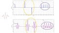
Figure 1 shows an example of such a convolution operation performed over two discrete time signals x1[n] = {2, 0, -1, 2} and x2[n] = {-1, 0, 1}. Here the first and the second rows correspond to the original signal x1[n] and flipped version of the signal x2[n], respectively.
.jpg)
Figure 1. Graphical method of finding convolution
Next, we have the third row which contains the product (values written in the blue font) of the overlapping samples from the first two rows. Finally, we can obtain the samples of the convoluted signal by adding these product terms, the corresponding values of which are represented by the red font in the figure.
Thus, in the example considered, we have our convoluted output signal to be y[n] = {-2, 0, 3, -2, -1, 2}.
Mathematical Expression
When defining any operation, it's helpful to express it in mathematical terms. Convolution is no exception!
Mathematically, the equation of convolution greatly resembles that of correlation. Unlike in correlation, however, convolution involves flipping one of the signals. This time-reversal can be represented as (t - τ), where τ is the time-instant considered.
As a result, for continuous time signals x1(t) and x2(t), we can express the convolution operation as
$$ y\left(t\right) = \int_{-\infty}^{\infty} \left\{x_{1}\left(\tau\right) x_{2}\left(t - \tau\right)\right\} d\tau $$
or
$$ y\left(t\right) = \int_{-\infty}^{\infty} \left\{x_{1}\left(t - \tau\right) x_{2}\left(\tau\right) \right\} d\tau $$
Equivalently, for discrete time signals, we have
$$ y\left[n\right] = \sum_{k = -\infty}^\infty \left\{ x_{1} \left[k\right] x_{2} \left[n-k\right]\right\} $$
or
$$ y\left[n\right] = \sum_{k = -\infty}^\infty \left\{ x_{1} \left[n-k\right] x_{2} \left[k\right] \right\} $$
Applications
Characterizing a linear time-invariant (LTI) system in terms of its transfer function
Consider a case where we're required to characterize an unknown system. This is important because it would help us gain an insight into the workings of the system. One way of characterizing a system is to express it in terms of its frequency transfer function, or its frequency spectrum.
To achieve this objective, a wide range of frequencies (generated by using sweep generators, for example) are imposed over the system one at a time and the response of the system for each of them is obtained. Provided we've maintained equal amplitude and phase for each and every frequency, we can conclude that any kind of amplitude and/or phase variations observed in the respective outputs are indicative of the system's characteristics. Thus, the cumulative result of these responses would be the frequency transfer function of the system.
However, there's one more way to tackle this issue. Recall that the Fourier transform of a delta function has a flat frequency spectrum with a constant value of 1 for the entire frequency range. This indicates that, instead of generating all the possible frequencies to impose on the system, one can use a single delta function as its input. In doing so, however, we've converted our frequency-domain issue into a time-domain issue.
This mode of change in the input signal also necessitates change in the operation performed over it. The new signal operation is convolution. This is because, per convolution theorem, multiplication in the frequency domain will take the form of convolution in the time domain, and multiplication in the time domain will take the form of convolution in the frequency domain.
So the result we obtain by using all the frequencies in frequency domain is the same as what we obtain by using delta function in conjunction with convolution operation in time domain.
A direct implication of this is a major application of convolution: characterization of a system in terms of its transfer function. Note that, if the system is linear and time-invariant (LTI), then its response to an impulse input is adequate for defining the characteristics of its transfer function (see Figure 2).
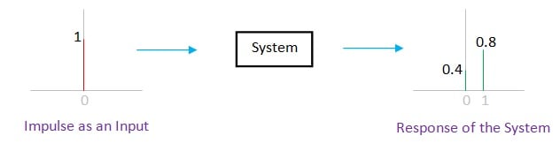
Figure 2. Characterizing the system in terms of its impulse response
Determining the output of an LTI system when its input is known
Consider a case where we have a system whose impulse response is as shown in Figure 2.
Now, let's assume this system to be linear and is fed by a single scaled impulse at its input. In this case, we can anticipate that the output of the system will be the same as the system’s response obtained in Figure 2, except being scaled by a degree equal to that of the input (right-most side of Figure 3).
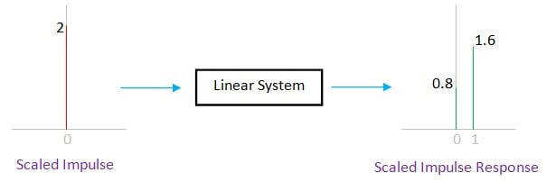
Figure 3. Response of a linear system for a scaled impulse at its input
Next, let's assume that the system exhibits the property of time-invariance. In such a case, if we provide it with an impulse which is shifted along the time axis, then the system will produce an output in which its impulse response is shifted by an equal amount (shown in Figure 4).
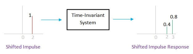
Figure 4. Response of a time-invariant system for a time-shifted impulse at its input
Now, what if the system is both linear as well as time-invariant? Just combine both the results!
If the system is LTI, then a scaled shifted impulse function at its input will yield a scaled shifted impulse response at its output (shown in Figure 5).

Figure 5. Response of an LTI system for a scaled, shifted impulse function
You might be wondering why we need to go over this. Before I answer, let's establish an important fact about signals that I hope most of you are familiar with: Any signal can be expressed in terms of unit impulses or dirac-delta functions. (Check out these resources for more information: Signals, Linear Systems, and Convolution and Signals in Natural Domain: Discrete-Time Convolution.)
Now, to get our answer, let's connect this concept to the discussion we've been having on convolution.
This fact about signal expression implies that any signal is a series of scaled impulse functions which are shifted in time. However, for each of these impulse functions, we can anticipate the system's behavior, provided we know its impulse response.
As LTI systems obey the law of superposition, we can add all these individual system responses. The result obtained through this process will be the output of the system when the input is fed to it.
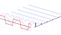
For example, an input signal {-1, 2, 1} can be split into three individual sequences: one of magnitude -1 positioned at time-instant 0, another of magnitude 2 positioned at time-instant 1, and the last one of magnitude 1 positioned at time-instant 2. This data is represented in tabular form in Table I of Figure 6.
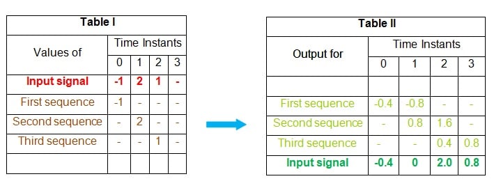
Figure 6. Finding the output of the system using convolution
Having put this information into table form, we can find the output of the system for each of these sequences separately. This is shown by the first three rows of Table II in Figure 6.
Lastly, we add the samples corresponding to each time-instant to get the overall output of the system (the last row of Table II). This result is the output of the system when fed by an input signal {-1, 2, 1}.
Essentially, we can effectively find the output of any LTI system by using convolution, provided we know its impulse response. Although the example above is of discrete domain signal, the statement holds good even for continuous time signals.
Summary
This article presents a brief introduction to convolution and the two scenarios in which it is widely used. Other fields in which convolution finds its application will be covered in Part II of this article series.
Related Content